The Calculus of Existence: A Mathematical Derivation of Life from Point Zero

Welcome to a comprehensive exploration of the mathematical foundations that underpin existence itself. This blog series, structured across three volumes, traces the journey from absolute nothingness to the complexity of consciousness and the infinite potential of the cosmos.

---

Table of Contents

Volume I: The Physical Build

• Chapter 1: Thermodynamics & The Null State
• Chapter 2: Reaction-Diffusion & The Origin of Form
• Chapter 3: Fractal Geometry & Efficiency
• Chapter 4: Evolutionary Game Theory

Volume II: The Biological Code

• Chapter 5: Chaos Theory and Adaptation
• Chapter 6: Information Theory & DNA
• Chapter 7: Neural Networks & Consciousness

Volume III: The Future

• Chapter 8: Bayesian Inference and Belief
• Chapter 9: Automata Theory and Artificial Life
• Chapter 10: The Drake Equation and The Cosmos

---

Introduction: The Null Hypothesis

To build life from "Point 0," we must first define it. In mathematics and physics, Point 0 is the Vacuum State or the state of Maximum Entropy. It is a condition where the probability of any specific organized structure (like a protein or a cell) existing is effectively zero.

The "Problem of Life" is a probability problem. If you take a box of Scrabble letters and dump them on the floor, the probability of them spelling the entire works of Shakespeare is so low it is considered impossible. Yet, life is exactly that: a pile of atoms that spontaneously arranged themselves into a structure capable of reading Shakespeare.

To prove how this happens, we must move through three mathematical phases:

1. Thermodynamics: The energy required to cheat randomness.
2. Reaction-Diffusion: The differential equations that create shape.
3. Information Theory: The code that preserves the shape.

---

Volume I: The Physical Build

Chapter 1: Thermodynamics & The Null State

Mathematical Domain: Statistical Mechanics
Key Concept: Negentropy & Gibbs Free Energy

We begin with the Second Law of Thermodynamics, the most ruthless law in physics. It states that the universe tends toward disorder.

1.1 The Boltzmann Definition

Ludwig Boltzmann defined the "messiness" of the universe (Entropy, $S$) with this equation:

$S = k_B \ln \Omega$

Where:

• $k_B$ is the Boltzmann constant ($1.38 \times 10^{-23} J/K$).
• $\Omega$ (Omega) is the number of possible "microstates" (ways atoms can be arranged).

At Point 0 (Dead Universe), $\Omega$ is maximized. The atoms are spread out evenly. To build a human, you need to force those atoms into a very specific, unlikely arrangement. This means you must decrease $\Omega$, which lowers Entropy ($S$). But the Second Law says $\Delta S_{total} > 0$. Disorder must increase.

1.2 The Schrödinger Escape Hatch

In 1944, physicist Erwin Schrödinger wrote What is Life?. He provided the mathematical proof that life does not violate the Second Law; it exploits a loophole. Life is an Open System. We are not a sealed box. We take in low-entropy energy (food/sunlight) and release high-entropy waste (heat).

The equation for a living system is:

$\Delta G = \Delta H - T\Delta S$

Where:

• $\Delta G$ is Gibbs Free Energy (The energy available to do work, i.e., "live").
• $\Delta H$ is Enthalpy (Heat content).
• $T$ is Temperature.
• $\Delta S$ is Entropy.

For a process to happen spontaneously (like a cell dividing), $\Delta G$ must be negative ($\Delta G < 0$). To keep building structure (lowering internal entropy, so $\Delta S$ is negative), the term $-T\Delta S$ becomes positive. To keep the total $\Delta G$ negative, you must burn massive amounts of fuel ($\Delta H$).

Mathematical Proof: Life is a localized combustion engine. We burn carbon to pay the "entropy tax" required to maintain our complex mathematical form. Without this energy flow, $S$ maximizes, and we reach "Point 0" again (Death).

---

Chapter 2: Reaction-Diffusion & The Origin of Form

Mathematical Domain: Partial Differential Equations (PDEs)
Key Concept: Turing Instability

Once we have energy, how do we get shape? Why is a blob of cells not just a sphere? Why do we have fingers, zebra stripes, or leopard spots? In 1952, Alan Turing (the father of the computer) published The Chemical Basis of Morphogenesis. He proved that you don't need a "God" or a "Master Builder" to create complex patterns. You only need two chemicals and simple calculus.

2.1 The Turing Equations

Imagine two chemicals in a "soup":

• Activator ($u$): Increases its own concentration and the concentration of the Inhibitor.
• Inhibitor ($v$): Decreases the concentration of the Activator.

Turing modeled their spread using these coupled Reaction-Diffusion Equations:

$\frac{\partial u}{\partial t} = D_u \nabla^2 u + f(u,v)$ $\frac{\partial v}{\partial t} = D_v \nabla^2 v + g(u,v)$

Breakdown of the Formula:

• $\frac{\partial u}{\partial t}$: How the concentration changes over time.
• $D_u \nabla^2 u$: The Diffusion Term. This describes how the chemical spreads out in space (like a drop of ink in water). $\nabla^2$ is the Laplacian operator, measuring the "smoothness" of the distribution.
• $f(u,v)$: The Reaction Term. This describes how the chemicals interact (e.g., $u$ makes more $u$, $v$ kills $u$).

2.2 The Stability Analysis

At Point 0, the mixture is uniform (gray soup). This is a "Homogeneous Steady State." Turing performed a Linear Stability Analysis on this state, looking for conditions where a tiny perturbation (random noise) would grow instead of fading away.

He discovered the condition for life: Differential Diffusion.

$D_v \gg D_u$

If the Inhibitor ($v$) diffuses much faster than the Activator ($u$), the system becomes unstable. The Activator creates a local "spot" of concentration, and the Inhibitor rushes out fast to suppress the surrounding area.

• Result: A spot is formed.
• Result: If you change the parameters slightly, the spots stretch into stripes.

This proves mathematically that a "Point 0" uniform blob must eventually develop structure (spots, stripes, limbs, segments) purely due to the laws of diffusion. No blueprint required.

---

Chapter 3: Fractal Geometry & Efficiency

Mathematical Domain: Fractal Geometry
Key Concept: Self-Similarity & Power Laws

Life has a scaling problem. A human body has 37 trillion cells. If you had to encode the position of every single cell in your DNA, your genome would be larger than the universe. Instead, nature uses Fractals.

3.1 The Fractal Dimension

Euclidean geometry (squares, circles) is too simple for life. Life is rough. A line is 1D, a plane is 2D. A rough, branching structure (like a lung or a tree) is somewhere in between. This is the Hausdorff Dimension ($D$):

$D = \frac{\log N}{\log (1/s)}$

Where:

• $N$ is the number of new self-similar pieces.
• $s$ is the scaling factor (how much smaller the new pieces are).

3.2 The Efficiency Proof

Why do lungs, blood vessels, and trees all look the same? Because they are solving the same mathematical optimization problem: Maximize Surface Area within a Minimal Volume.

If you build a lung using simple spheres, you get very little oxygen absorption. If you build it using a branching fractal (where the bronchus splits into bronchioles, which split again), you can pack the surface area of a tennis court (~75 m²) into the volume of a human chest (~6 liters).

This structure follows a mathematical Power Law:

$Y = Y_0 M^{3/4}$

(Kleiber’s Law: Metabolic rate scales to the 3/4 power of mass). This 1/4 scaling factor comes directly from the fractal geometry of our nutrient transport networks. We are built of fractals because it is the only way to be big and efficient simultaneously.

---

Chapter 4: Evolutionary Game Theory

Mathematical Domain: Game Theory & Optimization
Key Concept: Fitness Landscapes

Finally, how does "Point 0" become smart? We treat Evolution not as biology, but as an Optimization Algorithm running on a high-dimensional surface called a "Fitness Landscape."

4.1 The Replicator Equation

In Evolutionary Game Theory, we track the frequency ($x_i$) of a gene strategy $i$.

$\dot{x}_i = x_i (f_i(x) - \bar{f}(x))$

If the fitness of strategy $i$ ($f_i$) is greater than the average fitness of the population ($\bar{f}$), then the growth rate ($\dot{x}_i$) is positive. If it is lower, the strategy dies out.

4.2 Local vs. Global Maxima

Imagine a 3D mountain range. The "height" is survival. The population is a ball rolling around.

• Point 0: The bottom of the valley.
• Mutation: Pushes the ball in a random direction.
• Selection: Prevents the ball from rolling down.

Over millions of iterations ($t \rightarrow \infty$), the algorithm (Life) inevitably climbs the peaks. However, math shows a danger: Local Maxima. Sometimes a species gets stuck on a small hill (a "good enough" solution) and cannot cross the valley to get to the highest mountain (the "perfect" solution). This explains why biological flaws (like the human blind spot in the eye) exist. We are mathematically "stuck" at a local maximum.

---

SUMMARY OF VOLUME I

We have successfully moved from Point 0 to a Complex Organism using only math:

• Thermodynamics allows us to borrow order ($\Delta G < 0$).
• Turing Patterns allow us to break symmetry and form shapes ($D_v \gg D_u$).
• Fractals allow us to scale that shape efficiently ($D > 2$).
• Game Theory forces that shape to improve over time ($\dot{x} > 0$).

---

Volume II: From Chaos to Consciousness

In Volume I, we established how energy (Thermodynamics), shape (Turing Patterns), and structure (Fractals) arise from Point 0. Now, we must tackle the most difficult questions: How does life adapt? How does it remember? And how does it think? This volume covers the mathematics of Chaos, Information, and Intelligence.

Chapter 5: Chaos Theory and Adaptation

Mathematical Domain: Chaos Theory
Key Concept: The Bifurcation Diagram & Strange Attractors

Life cannot exist in a state of perfect order (crystals are dead) nor in perfect chaos (gas is dead). Life exists on a razor's edge known mathematically as the Edge of Chaos. This region allows for stability and adaptation.

5.1 The Logistic Map

To prove this, we look at the simplest mathematical model of population growth, the Logistic Map. It predicts the population ($x$) at the next time step ($n+1$) based on the current population ($x_n$) and a growth rate ($r$).

$x_{n+1} = r x_n (1 - x_n)$

Where $x_n$ is a number between 0 and 1 (where 1 is maximum population capacity).

5.2 The Road to Chaos

If we iterate this simple equation, the behavior changes drastically depending on $r$:

• Stagnation ($r < 3$): The system settles into a single, fixed number. (Life is static).
• Oscillation ($3 < r < 3.56$): The population cycles between 2, 4, or 8 values. (Life creates predictable seasons/heartbeats).
• Chaos ($r > 3.57$): The system becomes Deterministic Chaos. The output never repeats.

The Mathematical Proof: Life operates in the transition zone (The "Feigenbaum Point," $\delta \approx 4.669...$). This mathematical zone ensures that a small change in input (a mutation) can have a massive effect on the outcome (evolution). If life were perfectly stable, evolution would be mathematically impossible. We need chaos to evolve.

---

Chapter 6: Information Theory & DNA

Mathematical Domain: Information Theory
Key Concept: Shannon Entropy & Error Correction

Once a life form evolves a useful trait (like an eye), it must record that instruction. If it forgets, it dies. This brings us to Information Theory, founded by Claude Shannon.

6.1 Shannon Entropy

Shannon defined information not as "meaning," but as the resolution of uncertainty. The amount of information ($H$) in a genetic sequence is:

$H(X) = - \sum_{i=1}^{n} p(x_i) \log_2 p(x_i)$

Where $p(x_i)$ is the probability of a specific base pair appearing. DNA uses a quaternary (Base-4) system: A, C, T, G. Since there are 4 options, a single base pair holds: $\log_2(4) = 2$ bits of information. The human genome is roughly $3 \times 10^9$ base pairs. Mathematically, you are a data set of approximately 750 Megabytes (6 gigabits).

6.2 The Hamming Distance (Error Correction)

Life fights the "Noise" of the universe (radiation, chemical mistakes). If a bit flips (Mutation), the code breaks. To fix this, life uses Redundancy. In coding theory, the Hamming Distance ($d_{min}$) measures how different two valid codewords must be.

$d(x, y) = \sum |x_i - y_i|$

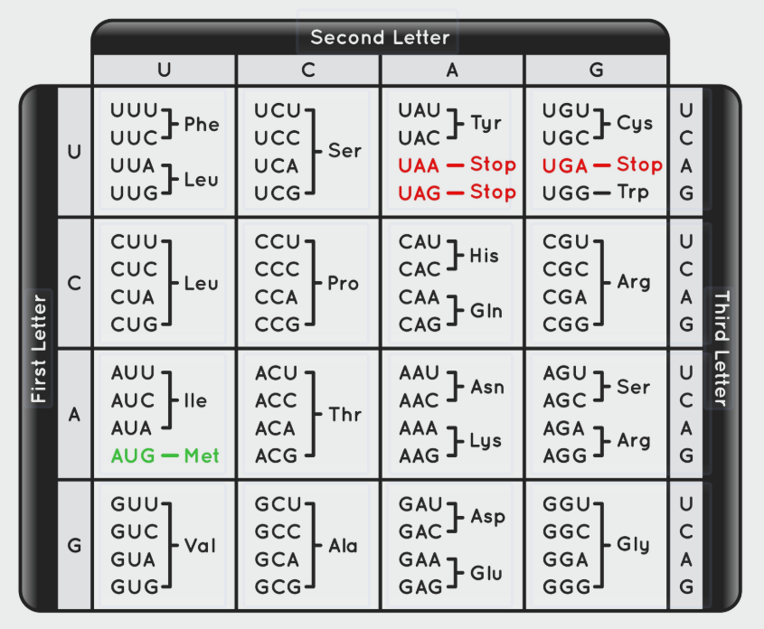
Life uses a triplet code (Codons): 3 DNA bases = 1 Amino Acid.

• Total combinations: $4^3 = 64$.
• Amino acids needed: 20.

The Mathematical Trick: Because $64 \gg 20$, there is massive redundancy. For example, the codons GGU, GGC, GGA, and GGG all code for Glycine. If the third bit is corrupted by radiation, the math protects the output. You still get Glycine. Life is built on Error-Correcting Code.

---

Chapter 7: Neural Networks & Consciousness

Mathematical Domain: Graph Theory & Linear Algebra
Key Concept: Emergence & Small-World Networks

Finally, we reach the brain. How does a collection of "dumb" neurons create "smart" consciousness? The answer lies in Network Topology.

7.1 The Perceptron (The Mathematical Neuron)

A single neuron is a simple mathematical function. It takes inputs ($x$), multiplies them by "weights" ($w$, importance), adds a bias ($b$), and pushes them through an activation function ($\sigma$).

$y = \sigma \left( \sum_{i=1}^{n} w_i x_i + b \right)$

This is a Linear Classifier. One neuron can make a simple decision (e.g., "Is it hot? Yes/No").

7.2 The Emergence of Intelligence

One neuron is useless. But if you layer them ($y_1 \rightarrow y_2 \rightarrow y_3$), the math changes. The Universal Approximation Theorem proves that a network of neurons with just one hidden layer can approximate any continuous function. This means a brain is not magic; it is a Function Approximator. It is mathematically solving for the function $f(x)$ where $x$ is sensory input and $f(x)$ is survival behavior.

7.3 Small-World Networks

Brain neurons connect via a specific graph topology called a Small-World Network. Defined by the Watts-Strogatz model, it balances:

• Clustering Coefficient ($C$): High local connectivity (specialized processing).
• Path Length ($L$): Short average distance between any two nodes.

The "Small-Worldness" ($S$) is defined as:

$S = \frac{C/C_{rand}}{L/L_{rand}} \gg 1$

This geometry allows the brain to synchronize globally (consciousness) while processing locally (vision, hearing). It is the most mathematically efficient way to wire a processor.

---

FINAL CONCLUSION: THE EQUATION OF LIFE

We have now traced the path from Point 0 to You:

• Thermodynamics ($\Delta G < 0$): Provided the energy to resist the void.
• Reaction-Diffusion ($D_v \gg D_u$): Sculpted the physical form.
• Fractals ($D > 2$): Optimized the biological space.
• Chaos ($r \approx 3.57$): Granted the flexibility to adapt.
• Information Theory ($H$): Encoded the blueprint in DNA.
• Network Theory ($S \gg 1$): Wired the mind.

Mathematical Q.E.D.
Life is not a violation of the universe's laws; it is a complex solution to them. We are the universe calculating itself.

---

Volume III: The Future of the Equation

We have covered Volume I (The Physical Build) and Volume II (The Biological Code). But to make this a complete mathematical proof of existence, we must look at where the math goes next: Artificial Intelligence and the Cosmos.

Chapter 8: Bayesian Inference and Belief

Mathematical Domain: Probability Theory
Key Concept: Predictive Coding

We established in Volume II that the brain is a network. But how does it actually learn about reality? It uses Bayes' Theorem. The brain is not a camera; it is a prediction engine. It constantly calculates the probability of a hypothesis ($H$) being true given new sensory data ($D$).

$P(H|D) = \frac{P(D|H) \cdot P(H)}{P(D)}$

• $P(H)$ (Prior): What you believe is true before seeing anything (e.g., "The sun will rise").
• $P(D|H)$ (Likelihood): The probability of seeing this data if your belief is true.
• $P(H|D)$ (Posterior): Your new updated belief after seeing the data.

The Free Energy Principle: Neuroscientist Karl Friston proved that all life tries to minimize "Free Energy" (Surprise). Mathematically, "Surprise" is the difference between your Prior ($P(H)$) and the Reality ($D$).

$F = - \ln P(D|H) - \text{Complexity}$

Life creates models of the world to minimize $F$. If $F$ gets too high, the organism dies because its internal math no longer matches external reality.

---

Chapter 9: Automata Theory and Artificial Life

Mathematical Domain: Automata Theory
Key Concept: The Universal Constructor

Can we build life from scratch? John von Neumann (who also invented the computer architecture we use today) proved the possibility of a Universal Constructor ($U_c$). For an object to reproduce, it needs three parts:

1. The Blueprint ($B$): The code (DNA).
2. The Factory ($F$): The machine that reads $B$ to build a copy of the machine.
3. The Copier ($C$): The machine that copies $B$ itself to put into the new machine.

$U_c + B \rightarrow U_c + B + (U_c + B)$

The Paradox Solved: Before Von Neumann, it was thought that a machine could only build something simpler than itself (entropy). Von Neumann proved mathematically that if a system reaches a specific threshold of complexity, it can build a system equal to or more complex than itself. This is the mathematical proof that AI can eventually build better AI, leading to a singularity.

---

Chapter 10: The Drake Equation and The Cosmos

Mathematical Domain: Astrophysics / Probability
Key Concept: The Great Filter

Does this math happen elsewhere? The Drake Equation attempts to quantify the number of active, communicating civilizations in our galaxy ($N$).

$N = R_* \cdot f_p \cdot n_e \cdot f_l \cdot f_i \cdot f_c \cdot L$

• $R_*$: Rate of star formation.
• $f_p$: Fraction of those stars with planets.
• $n_e$: Number of planets that could support life (Habitable Zone).
• $f_l$: Fraction where life actually develops (The Thermodynamics step).
• $f_i$: Fraction where intelligence develops (The Network step).
• $f_c$: Fraction that communicates (Radio/Lasers).
• $L$: How long they survive.

The Mathematical Terror: We have not heard from anyone (The Fermi Paradox). This implies that one of the variables in the equation is close to zero. Is it $f_l$ (Is starting life mathematically impossible?) or is it $L$ (Does every civilization destroy itself with nuclear math?)?

---

Epilogue: The Omega Point

The Final Limit

We started at Point 0 (Maximum Entropy), moved through Life (Negative Entropy), and are moving toward The Omega Point (Maximum Complexity). Pierre Teilhard de Chardin and later physicist Frank Tipler proposed that the universe is a computer processing information. As life spreads (via Von Neumann probes) and converts dead matter into thinking matter ("Computronium"), the universe wakes up.

The final equation of existence is not a static number. It is a limit function:

$\lim_{t \to \infty} \text{Intelligence}(t) = \infty$

The Proof is Complete.
You have moved from the stillness of the void, through the chaos of chemistry, into the structure of biology, the order of the mind, and finally, into the infinite potential of the future.