Why Senior Engineers Master Raw SQL and why ORMs aren't enough

📖 Introduction

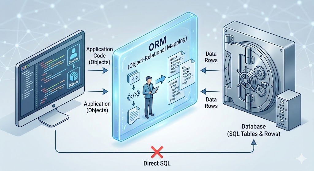
At the junior or intermediate level, Object-Relational Mappers (ORMs) like Hibernate, TypeORM, or Sequelize are saviors. They abstract away the database, letting you treat rows like objects. However, as systems scale to millions of requests, the "Magic" of the ORM becomes a liability.

This guide details 15 specific technical areas where ORMs fail and raw SQL knowledge is required to maintain performance, data integrity, and architectural sanity.

📑 Table of Contents

The Leakiness of Abstractions
The Infamous N+1 Problem
Complex Joins & Cartesian Explosions
Window Functions for Analytics
Recursive CTEs (Common Table Expressions)
Bulk Operations & Performance
Database-Specific Types (JSONB, Arrays)
Fine-Grained Locking & Concurrency
Understanding Execution Plans (EXPLAIN ANALYZE)
Materialized Views for Caching
Subquery Optimization
Composite Indexes & Index Utilization
Set Operations (UNION, INTERSECT)
Data Migration & Schema Evolution
The Hybrid Approach (The Senior Solution)

1. The Leakiness of Abstractions

The Fundamental Problem

Concept: Spolsky's Law of Leaky Abstractions states that "All non-trivial abstractions, to some degree, are leaky." ORMs promise to hide SQL complexity, but when things break, you need to understand what's happening at the database level.

Explanation: When an ORM throws an error or creates a slow request, it doesn't return a Java/Python error; it returns a database timeout, a locking error, or a cryptic constraint violation. You cannot fix what you cannot understand.

Real Scenario: The Deadlock Mystery

Your e-commerce app crashes during Black Friday. The logs show:

ERROR: Deadlock found when trying to get lock; try restarting transaction

ORM Code (Django/SQLAlchemy-style):

# Payment processing endpoint - looks innocent
with transaction.atomic():
    user = User.objects.get(id=user_id)
    user.balance -= 100
    user.save()
    
    order = Order.objects.get(id=order_id)
    order.status = "PAID"
    order.save()

What Actually Happens Under Load:

Two concurrent requests process payments for the same user:

Request A Timeline:

-- T1: Request A starts
BEGIN;
SELECT * FROM users WHERE id = 123 FOR UPDATE;  -- Locks user row
UPDATE users SET balance = balance - 100 WHERE id = 123;

-- T2: Waiting to lock order...
SELECT * FROM orders WHERE id = 456 FOR UPDATE;  -- Waiting...

Request B Timeline:

-- T1.5: Request B starts (slightly offset)
BEGIN;
SELECT * FROM orders WHERE id = 456 FOR UPDATE;  -- Locks order row
UPDATE orders SET status = 'PAID' WHERE id = 456;

-- T2.5: Waiting to lock user...
SELECT * FROM users WHERE id = 123 FOR UPDATE;  -- DEADLOCK!

The Deadlock Cycle:

Request A holds lock on users(123), waits for orders(456)
Request B holds lock on orders(456), waits for users(123)
Database detects circular dependency and kills one transaction

The Leak: What ORMs Don't Hide

The ORM abstraction breaks down because it cannot hide:

Row-level locks - SELECT ... FOR UPDATE is implicit
Transaction isolation levels - READ COMMITTED vs SERIALIZABLE
Lock ordering - The sequence of row access matters
Lock escalation - Row locks can escalate to table locks
Gap locks - InnoDB locks ranges, not just rows
MVCC behavior - Multi-Version Concurrency Control nuances

Who Can Fix It?

❌ ORM-only Developer:

# Tries to catch the exception and retry
try:
    with transaction.atomic():
        user.balance -= 100
        user.save()
        order.status = "PAID"
        order.save()
except DatabaseError:
    # Retry? How many times? This doesn't fix the root cause!
    pass

✅ SQL Expert - Solution 1: Consistent Lock Ordering

# Always acquire locks in the same order: users first, then orders
with transaction.atomic():
    # Force lock acquisition order
    user = User.objects.select_for_update().get(id=user_id)
    order = Order.objects.select_for_update().get(id=order_id)
    
    user.balance -= 100
    user.save()
    order.status = "PAID"
    order.save()

Generated SQL:

BEGIN;
SELECT * FROM users WHERE id = 123 FOR UPDATE;      -- Lock 1
SELECT * FROM orders WHERE id = 456 FOR UPDATE;     -- Lock 2
UPDATE users SET balance = balance - 100 WHERE id = 123;
UPDATE orders SET status = 'PAID' WHERE id = 456;
COMMIT;

✅ SQL Expert - Solution 2: Single Atomic Statement

-- Even better: Use a single UPDATE with JOIN (PostgreSQL)
BEGIN;
UPDATE users u
SET balance = u.balance - 100
FROM orders o
WHERE u.id = 123 
  AND o.id = 456 
  AND o.user_id = u.id
RETURNING u.balance, o.status;

UPDATE orders SET status = 'PAID' WHERE id = 456;
COMMIT;

✅ SQL Expert - Solution 3: Adjust Isolation Level

# For read-heavy workloads, use READ COMMITTED instead of SERIALIZABLE
from django.db import connection

with connection.cursor() as cursor:
    cursor.execute("SET TRANSACTION ISOLATION LEVEL READ COMMITTED")
    
with transaction.atomic():
    # Your transaction logic here
    pass

Transaction Isolation Levels Deep Dive

Isolation Level	Dirty Read	Non-Repeatable Read	Phantom Read	Performance
READ UNCOMMITTED	✅ Possible	✅ Possible	✅ Possible	Fastest
READ COMMITTED	❌ Prevented	✅ Possible	✅ Possible	Fast
REPEATABLE READ	❌ Prevented	❌ Prevented	✅ Possible	Moderate
SERIALIZABLE	❌ Prevented	❌ Prevented	❌ Prevented	Slowest

Example: Non-Repeatable Read Problem

# ORM code that seems safe but isn't
with transaction.atomic():
    user = User.objects.get(id=123)
    initial_balance = user.balance  # Read 1: $1000
    
    # Another transaction updates the balance here!
    
    user = User.objects.get(id=123)
    current_balance = user.balance  # Read 2: $500 (DIFFERENT!)
    
    # Logic breaks because we expected consistent reads
    if initial_balance != current_balance:
        raise InconsistentStateError()

SQL Expert Fix:

-- Use REPEATABLE READ or explicit locking
SET TRANSACTION ISOLATION LEVEL REPEATABLE READ;
BEGIN;
SELECT balance FROM users WHERE id = 123;  -- Always returns same value
-- ... other operations ...
SELECT balance FROM users WHERE id = 123;  -- Guaranteed same result
COMMIT;

Real Production Debugging Story

Symptom: Random IntegrityError: duplicate key value violates unique constraint on high-traffic endpoint.

ORM Code:

# Looks safe - checking before insert
if not User.objects.filter(email=email).exists():
    User.objects.create(email=email)  # Still fails sometimes!

The Race Condition:

Time    Request A                           Request B
----    ---------                           ---------
T1      SELECT COUNT(*) FROM users 
        WHERE email='x@y.com'  (0 rows)
        
T2                                          SELECT COUNT(*) FROM users
                                            WHERE email='x@y.com'  (0 rows)
        
T3      INSERT INTO users (email) 
        VALUES ('x@y.com')  ✅
        
T4                                          INSERT INTO users (email)
                                            VALUES ('x@y.com')  ❌ DUPLICATE!

SQL Expert Solution:

-- Use INSERT ... ON CONFLICT (PostgreSQL 9.5+)
INSERT INTO users (email, name) 
VALUES ('x@y.com', 'John')
ON CONFLICT (email) DO NOTHING
RETURNING id;

-- Or use a unique constraint with proper error handling
-- Or use SELECT ... FOR UPDATE in a transaction
BEGIN;
SELECT id FROM users WHERE email = 'x@y.com' FOR UPDATE;
-- If not exists, then insert
INSERT INTO users (email) VALUES ('x@y.com');
COMMIT;

Django ORM Equivalent (requires SQL knowledge to use):

from django.db import IntegrityError

try:
    user = User.objects.create(email=email)
except IntegrityError:
    user = User.objects.get(email=email)

# Or better, use get_or_create with proper understanding
user, created = User.objects.get_or_create(
    email=email,
    defaults={'name': 'John'}
)

Key Takeaway

ORMs are excellent tools, but they're leaky abstractions. When you encounter:

Deadlocks
Race conditions
Performance issues
Constraint violations
Timeout errors

You must understand the underlying SQL to diagnose and fix the problem. The ORM won't save you.

2. The Infamous N+1 Problem

The Silent Performance Killer

Concept: Fetching a parent object and then iterating to fetch its children results in 1 initial query + N queries for children. With 100 users, that's 101 database round trips.

Why It's Dangerous:

Often invisible in development (small datasets)
Exponentially worse with nested relationships
Network latency multiplies the problem
Can bring production systems to their knees

Example 1: Basic N+1 Query

ORM Code (Inefficient):

# Django Example - Looks innocent
users = User.objects.all()  # Query 1: SELECT * FROM users
for user in users:
    print(user.profile.address)  # Query 2-101: SELECT * FROM profiles WHERE user_id = ?

Generated SQL (100 users = 101 queries):

-- Query 1
SELECT id, name, email FROM users;

-- Query 2
SELECT address FROM profiles WHERE user_id = 1;

-- Query 3
SELECT address FROM profiles WHERE user_id = 2;

-- ... 98 more queries ...

-- Query 101
SELECT address FROM profiles WHERE user_id = 100;

Performance Impact:

Database Time: 101 queries × 5ms = 505ms
Network Latency: 101 round trips × 2ms = 202ms
Total: ~700ms for a simple list operation

Raw SQL Solution:

SELECT u.id, u.name, u.email, p.address
FROM users u
LEFT JOIN profiles p ON u.id = p.user_id;
-- 1 Query total: ~10ms

Performance Gain: 700ms → 10ms = 70x faster

Example 2: Nested N+1 (The Nightmare)

Scenario: Display users, their posts, and comments on each post.

ORM Code:

# Django/SQLAlchemy style
users = User.objects.all()  # 1 query
for user in users:  # 100 users
    print(f"User: {user.name}")
    for post in user.posts.all():  # 100 queries (1 per user)
        print(f"  Post: {post.title}")
        for comment in post.comments.all():  # 500 queries (5 posts per user)
            print(f"    Comment: {comment.text}")

Query Count Explosion:

1 (users) 
+ 100 (posts per user) 
+ 500 (comments per post) 
= 601 QUERIES! 🔥

Execution Time: 601 queries × 7ms = 4.2 seconds

Raw SQL Solution:

SELECT 
    u.id as user_id,
    u.name as user_name,
    p.id as post_id,
    p.title as post_title,
    c.id as comment_id,
    c.text as comment_text
FROM users u
LEFT JOIN posts p ON u.id = p.user_id
LEFT JOIN comments c ON p.id = c.post_id
ORDER BY u.id, p.id, c.id;
-- 1 query: ~25ms

Performance Gain: 4200ms → 25ms = 168x faster

Example 3: Real-World E-Commerce API

Endpoint: GET /api/products - List products with categories, reviews, and seller info

Naive ORM Implementation:

# Flask + SQLAlchemy
@app.route('/api/products')
def get_products():
    products = Product.query.limit(50).all()  # Query 1
    result = []
    
    for product in products:  # 50 iterations
        result.append({
            'name': product.name,
            'category': product.category.name,  # Query 2-51
            'seller': product.seller.company_name,  # Query 52-101
            'avg_rating': sum(r.rating for r in product.reviews) / len(product.reviews),  # Query 102-151
            'review_count': len(product.reviews)  # Already fetched above
        })
    
    return jsonify(result)

Total Queries: 1 + 50 + 50 + 50 = 151 queries

Execution Time: 151 × 8ms = 1.2 seconds (unacceptable for an API)

ORM Solution with Eager Loading:

from sqlalchemy.orm import joinedload

@app.route('/api/products')
def get_products():
    products = Product.query\
        .options(
            joinedload(Product.category),
            joinedload(Product.seller),
            joinedload(Product.reviews)
        )\
        .limit(50)\
        .all()  # Now just 1 query with joins
    
    result = []
    for product in products:
        result.append({
            'name': product.name,
            'category': product.category.name,  # No extra query!
            'seller': product.seller.company_name,  # No extra query!
            'avg_rating': sum(r.rating for r in product.reviews) / len(product.reviews) if product.reviews else 0,
            'review_count': len(product.reviews)
        })
    
    return jsonify(result)

Generated SQL:

SELECT 
    products.id, products.name, products.price,
    categories.id, categories.name,
    sellers.id, sellers.company_name,
    reviews.id, reviews.rating, reviews.text
FROM products
LEFT JOIN categories ON products.category_id = categories.id
LEFT JOIN sellers ON products.seller_id = sellers.id
LEFT JOIN reviews ON products.id = reviews.product_id
WHERE products.id IN (/* 50 product IDs */)
LIMIT 50;

Execution Time: ~35ms = 34x faster

Example 4: Even Better - Raw SQL with Aggregation

Problem with ORM Eager Loading: Still fetches ALL reviews, even though we only need count and average.

Optimized Raw SQL:

SELECT 
    p.id,
    p.name,
    p.price,
    c.name as category_name,
    s.company_name as seller_name,
    COUNT(r.id) as review_count,
    COALESCE(AVG(r.rating), 0) as avg_rating
FROM products p
LEFT JOIN categories c ON p.category_id = c.id
LEFT JOIN sellers s ON p.seller_id = s.id
LEFT JOIN reviews r ON p.id = r.product_id
GROUP BY p.id, p.name, p.price, c.name, s.company_name
LIMIT 50;

Execution Time: ~15ms = 80x faster than naive ORM

Data Transfer:

ORM with eager loading: ~500KB (all review text)
Optimized SQL: ~5KB (just aggregates)

Framework-Specific Solutions

Django

# Bad
users = User.objects.all()
for user in users:
    print(user.profile.bio)  # N+1!

# Good - select_related (for ForeignKey/OneToOne)
users = User.objects.select_related('profile').all()
for user in users:
    print(user.profile.bio)  # No extra queries

# Good - prefetch_related (for ManyToMany/Reverse FK)
users = User.objects.prefetch_related('posts').all()
for user in users:
    for post in user.posts.all():  # No extra queries
        print(post.title)

TypeORM (Node.js)

// Bad
const users = await userRepository.find();
for (const user of users) {
    console.log(user.profile.address);  // N+1!
}

// Good
const users = await userRepository.find({
    relations: ['profile', 'posts', 'posts.comments']
});
for (const user of users) {
    console.log(user.profile.address);  // Loaded!
}

Hibernate (Java)

// Bad
List<User> users = session.createQuery("FROM User", User.class).list();
for (User user : users) {
    System.out.println(user.getProfile().getAddress());  // N+1!
}

// Good - JOIN FETCH
List<User> users = session.createQuery(
    "SELECT u FROM User u LEFT JOIN FETCH u.profile", 
    User.class
).list();

Entity Framework (C#)

// Bad
var users = context.Users.ToList();
foreach (var user in users) {
    Console.WriteLine(user.Profile.Address);  // N+1!
}

// Good - Include
var users = context.Users
    .Include(u => u.Profile)
    .Include(u => u.Posts)
        .ThenInclude(p => p.Comments)
    .ToList();

Detection Tools

1. Django Debug Toolbar

# Shows all queries with duplicates highlighted
# Install: pip install django-debug-toolbar

2. SQLAlchemy Echo

engine = create_engine('postgresql://...', echo=True)
# Prints all SQL to console

3. npx-query-monitor (Node.js)

npm install --save-dev query-monitor
# Detects N+1 queries in development

4. Bullet Gem (Ruby on Rails)

# Gemfile
gem 'bullet', group: 'development'

# Raises errors on N+1 queries

The Hidden Cost: Network Latency

Scenario: Database on AWS RDS, App on EC2 in same region

Queries	DB Time (5ms each)	Network (2ms each)	Total Time
1	5ms	2ms	7ms
10	50ms	20ms	70ms
100	500ms	200ms	700ms
1000	5000ms	2000ms	7000ms

Cross-region latency (50ms):

100 queries = 100 × 50ms = 5 seconds just in network time!

Real Production War Story

Company: SaaS platform with 10K users
Symptom: Dashboard loading takes 45 seconds
Root Cause: N+1 queries fetching user permissions

Before (ORM):

def get_dashboard_data(user_id):
    user = User.objects.get(id=user_id)  # 1 query
    
    widgets = []
    for widget in Widget.objects.all():  # 1 query, 200 widgets
        if user.has_permission(widget.required_permission):  # 200 queries!
            widgets.append(widget)
    
    return widgets

Query Count: 1 + 1 + 200 = 202 queries
Time: 45 seconds

After (Raw SQL):

SELECT w.*
FROM widgets w
WHERE EXISTS (
    SELECT 1 
    FROM user_permissions up
    WHERE up.user_id = $1
      AND up.permission_id = w.required_permission_id
);

Query Count: 1 query
Time: 120ms
Improvement: 375x faster

Key Takeaways

Always use eager loading when you know you'll access related data
Monitor query counts in development with debug tools
Prefer aggregation in SQL over fetching all data and computing in code
Network latency matters - minimize round trips
Test with production-sized datasets - N+1 is invisible with 10 rows

3. Complex Joins & Cartesian Explosions

The Problem with Multi-Table Queries

Concept: ORMs often struggle to construct efficient joins across 4+ tables, sometimes defaulting to inefficient subqueries or fetching too much data in memory. Worse, they can create Cartesian products that multiply row counts exponentially.

SQL Advantage: You can explicitly control the JOIN order, type (LEFT vs INNER), and filtering strategy to prevent the database from loading millions of rows into memory.

Understanding Cartesian Explosions

Scenario: Fetching orders with multiple items AND multiple shipments.

Data:

1 Order
3 OrderItems (for that order)
2 Shipments (for that order)

Naive JOIN Result:

SELECT *
FROM orders o
LEFT JOIN order_items oi ON o.id = oi.order_id
LEFT JOIN shipments s ON o.id = s.order_id;

Result Set: 3 × 2 = 6 rows (Cartesian product!)

order_id | item_id | item_name | shipment_id | tracking
---------|---------|-----------|-------------|----------
1        | 101     | Widget A  | 501         | TRACK001
1        | 101     | Widget A  | 502         | TRACK002  ← Duplicate item!
1        | 102     | Widget B  | 501         | TRACK001  ← Duplicate item!
1        | 102     | Widget B  | 502         | TRACK002  ← Duplicate item!
1        | 103     | Widget C  | 501         | TRACK001  ← Duplicate item!
1        | 103     | Widget C  | 502         | TRACK002  ← Duplicate item!

With 100 items and 50 shipments: 100 × 50 = 5,000 rows for a single order!

Real-World Example: E-Commerce Report

Requirement: Generate a report showing Orders → OrderItems → Products → Categories → Warehouses → Shippers

ORM Attempt (Django):

# This looks reasonable but is a disaster
orders = Order.objects.select_related(
    'customer',
    'shipper'
).prefetch_related(
    'items__product__category',
    'items__product__warehouse',
    'shipments'
).all()

for order in orders:
    print(f"Order {order.id}")
    for item in order.items.all():
        print(f"  Item: {item.product.name}")
        print(f"  Category: {item.product.category.name}")
        print(f"  Warehouse: {item.product.warehouse.location}")
    for shipment in order.shipments.all():
        print(f"  Shipment: {shipment.tracking_number}")

Generated SQL (Simplified):

-- Query 1: Orders with customer and shipper
SELECT * FROM orders o
LEFT JOIN customers c ON o.customer_id = c.id
LEFT JOIN shippers sh ON o.shipper_id = sh.id;

-- Query 2: Order items (prefetch)
SELECT * FROM order_items WHERE order_id IN (1,2,3,...);

-- Query 3: Products (prefetch)
SELECT * FROM products WHERE id IN (101,102,103,...);

-- Query 4: Categories (prefetch)
SELECT * FROM categories WHERE id IN (10,11,12,...);

-- Query 5: Warehouses (prefetch)
SELECT * FROM warehouses WHERE id IN (20,21,22,...);

-- Query 6: Shipments (prefetch)
SELECT * FROM shipments WHERE order_id IN (1,2,3,...);

Total Queries: 6 (better than N+1, but still multiple round trips)

Problem: If you have 1000 orders, you're still doing 6 database round trips with large IN clauses.

SQL Expert Solution 1: Separate Aggregations

Strategy: Query items and shipments separately, then merge in application code.

-- Query 1: Orders with items
SELECT 
    o.id as order_id,
    o.order_date,
    c.name as customer_name,
    oi.id as item_id,
    p.name as product_name,
    cat.name as category_name,
    w.location as warehouse_location,
    oi.quantity,
    oi.price
FROM orders o
LEFT JOIN customers c ON o.customer_id = c.id
LEFT JOIN order_items oi ON o.id = oi.order_id
LEFT JOIN products p ON oi.product_id = p.id
LEFT JOIN categories cat ON p.category_id = cat.id
LEFT JOIN warehouses w ON p.warehouse_id = w.id
WHERE o.order_date >= '2024-01-01'
ORDER BY o.id, oi.id;

-- Query 2: Shipments (separate to avoid Cartesian product)
SELECT 
    s.order_id,
    s.tracking_number,
    s.shipped_date,
    sh.company_name as shipper_name
FROM shipments s
LEFT JOIN shippers sh ON s.shipper_id = sh.id
WHERE s.order_id IN (SELECT id FROM orders WHERE order_date >= '2024-01-01')
ORDER BY s.order_id;

Total Queries: 2 (vs 6 with ORM)
Cartesian Product: Avoided
Application Code: Merge results by order_id

SQL Expert Solution 2: JSON Aggregation (PostgreSQL)

Strategy: Use json_agg() to group related data into JSON arrays.

SELECT 
    o.id,
    o.order_date,
    o.total_amount,
    json_build_object(
        'id', c.id,
        'name', c.name,
        'email', c.email
    ) as customer,
    
    -- Aggregate order items into JSON array
    COALESCE(
        json_agg(
            DISTINCT jsonb_build_object(
                'item_id', oi.id,
                'product_name', p.name,
                'category', cat.name,
                'warehouse', w.location,
                'quantity', oi.quantity,
                'price', oi.price
            )
        ) FILTER (WHERE oi.id IS NOT NULL),
        '[]'
    ) as items,
    
    -- Aggregate shipments into separate JSON array
    COALESCE(
        (
            SELECT json_agg(
                json_build_object(
                    'tracking', s.tracking_number,
                    'shipped_date', s.shipped_date,
                    'shipper', sh.company_name
                )
            )
            FROM shipments s
            LEFT JOIN shippers sh ON s.shipper_id = sh.id
            WHERE s.order_id = o.id
        ),
        '[]'
    ) as shipments

FROM orders o
LEFT JOIN customers c ON o.customer_id = c.id
LEFT JOIN order_items oi ON o.id = oi.order_id
LEFT JOIN products p ON oi.product_id = p.id
LEFT JOIN categories cat ON p.category_id = cat.id
LEFT JOIN warehouses w ON p.warehouse_id = w.id
WHERE o.order_date >= '2024-01-01'
GROUP BY o.id, c.id, c.name, c.email
ORDER BY o.id;

Result (Single Row per Order):

{
  "id": 1,
  "order_date": "2024-01-15",
  "total_amount": 299.99,
  "customer": {
    "id": 42,
    "name": "John Doe",
    "email": "john@example.com"
  },
  "items": [
    {
      "item_id": 101,
      "product_name": "Widget A",
      "category": "Electronics",
      "warehouse": "NYC",
      "quantity": 2,
      "price": 99.99
    },
    {
      "item_id": 102,
      "product_name": "Widget B",
      "category": "Electronics",
      "warehouse": "LA",
      "quantity": 1,
      "price": 149.99
    }
  ],
  "shipments": [
    {
      "tracking": "TRACK001",
      "shipped_date": "2024-01-16",
      "shipper": "FedEx"
    },
    {
      "tracking": "TRACK002",
      "shipped_date": "2024-01-17",
      "shipper": "UPS"
    }
  ]
}

Benefits:

1 query instead of 6
No Cartesian product - each order is 1 row
Perfect for APIs - JSON output ready to send
Reduced network transfer - no duplicate data

Performance Comparison

Dataset:

10,000 orders
Average 5 items per order
Average 2 shipments per order

Approach	Queries	Rows Returned	Transfer Size	Time
Naive ORM (N+1)	30,001	60,000	15 MB	8.5s
ORM Prefetch	6	60,000	15 MB	450ms
Raw SQL (2 queries)	2	60,000	12 MB	180ms
Raw SQL (JSON agg)	1	10,000	8 MB	95ms

Join Order Optimization

Problem: The database query planner doesn't always choose the optimal join order.

Example: Inefficient Join Order

-- Bad: Joins large tables first, then filters
SELECT *
FROM orders o
JOIN order_items oi ON o.id = oi.order_id  -- 1M rows
JOIN products p ON oi.product_id = p.id    -- 1M rows
WHERE o.customer_id = 123                   -- Filters to 10 rows at the end!
  AND o.order_date >= '2024-01-01';

Execution Plan:

Hash Join  (cost=50000..80000 rows=1000000)
  -> Seq Scan on order_items  (1000000 rows)
  -> Hash
    -> Seq Scan on products  (100000 rows)
  -> Filter: customer_id = 123  (applied late!)

Optimized: Filter Early

-- Good: Filter first, then join
SELECT *
FROM (
    SELECT * 
    FROM orders 
    WHERE customer_id = 123 
      AND order_date >= '2024-01-01'
) o
JOIN order_items oi ON o.id = oi.order_id
JOIN products p ON oi.product_id = p.id;

Or use CTE for clarity:

WITH filtered_orders AS (
    SELECT id, order_date, total_amount
    FROM orders
    WHERE customer_id = 123
      AND order_date >= '2024-01-01'
)
SELECT 
    o.*,
    oi.quantity,
    p.name as product_name
FROM filtered_orders o
JOIN order_items oi ON o.id = oi.order_id
JOIN products p ON oi.product_id = p.id;

Execution Plan (Optimized):

Nested Loop  (cost=10..500 rows=10)
  -> Index Scan on orders  (10 rows) ← Filtered early!
  -> Index Scan on order_items  (50 rows)
  -> Index Scan on products  (50 rows)

Performance: 80,000 cost → 500 cost = 160x faster

Advanced: LATERAL Joins (PostgreSQL)

Problem: For each order, get the 3 most recent shipments.

ORM Approach: Impossible without raw SQL or post-processing.

SQL Solution:

SELECT 
    o.id,
    o.order_date,
    recent_shipments.tracking_number,
    recent_shipments.shipped_date
FROM orders o
CROSS JOIN LATERAL (
    SELECT tracking_number, shipped_date
    FROM shipments s
    WHERE s.order_id = o.id
    ORDER BY s.shipped_date DESC
    LIMIT 3
) recent_shipments
WHERE o.order_date >= '2024-01-01';

Use Case: Top N per group without window functions.

MySQL vs PostgreSQL Join Differences

MySQL (before 8.0):

No FULL OUTER JOIN
Must use UNION to simulate

-- PostgreSQL
SELECT * FROM a FULL OUTER JOIN b ON a.id = b.id;

-- MySQL workaround
SELECT * FROM a LEFT JOIN b ON a.id = b.id
UNION
SELECT * FROM a RIGHT JOIN b ON a.id = b.id;

PostgreSQL Advantages:

LATERAL joins
DISTINCT ON
Better query planner for complex joins

Real Production Debugging

Symptom: Report query times out after 30 seconds.

Query:

SELECT *
FROM orders o
JOIN customers c ON o.customer_id = c.id
JOIN order_items oi ON o.id = oi.order_id
JOIN products p ON oi.product_id = p.id
JOIN categories cat ON p.category_id = cat.id
WHERE cat.name = 'Electronics';

EXPLAIN ANALYZE Output:

Hash Join  (cost=100000..500000 rows=1000000)
  -> Seq Scan on order_items  (cost=0..50000 rows=1000000)
  -> Hash
    -> Seq Scan on products  (cost=0..30000 rows=100000)
    -> Seq Scan on categories  (cost=0..100 rows=10)

Problem: Scanning all 1M order_items before filtering by category!

Fix: Rewrite with Subquery

-- Filter products first
WITH electronics_products AS (
    SELECT p.id
    FROM products p
    JOIN categories cat ON p.category_id = cat.id
    WHERE cat.name = 'Electronics'
)
SELECT 
    o.*,
    c.name as customer_name,
    oi.quantity,
    p.name as product_name
FROM electronics_products ep
JOIN order_items oi ON oi.product_id = ep.id
JOIN orders o ON oi.order_id = o.id
JOIN customers c ON o.customer_id = c.id
JOIN products p ON oi.product_id = p.id;

New Execution Plan:

Nested Loop  (cost=50..5000 rows=1000)
  -> Index Scan on categories  (1 row) ← Start here!
  -> Index Scan on products  (5000 rows)
  -> Index Scan on order_items  (10000 rows)

Performance: 30 seconds → 200ms = 150x faster

Key Takeaways

Understand Cartesian products - they multiply row counts exponentially
Use JSON aggregation (PostgreSQL) to avoid Cartesian explosions
Filter early - push WHERE clauses as close to the source as possible
Control join order with CTEs or subqueries when the planner fails
Use EXPLAIN ANALYZE to verify the execution plan
Separate queries can be faster than one complex query with Cartesian products

4. Window Functions for Analytics

The Power of Window Functions

Concept: Window functions perform calculations across a set of table rows that are somehow related to the current row, without collapsing rows like GROUP BY does. They're essential for:

Running totals and moving averages
Ranking and percentiles
Lead/lag comparisons
Top N per group
Gap and island detection

ORM Limitation: Most ORMs do not support window functions natively. You end up pulling all data to the app server and calculating in loops (slow, memory-intensive, error-prone).

Example 1: Ranking - Top Sellers per Category

Business Requirement: Show each product with its rank within its category by sales.

ORM Approach (Inefficient):

# Django/Python - fetch everything and rank in memory
from collections import defaultdict

products = Product.objects.select_related('category').all()

# Group by category
by_category = defaultdict(list)
for product in products:
    by_category[product.category.id].append(product)

# Sort and rank each category
results = []
for category_id, products_list in by_category.items():
    sorted_products = sorted(products_list, key=lambda p: p.total_sales, reverse=True)
    for rank, product in enumerate(sorted_products, 1):
        results.append({
            'product': product.name,
            'category': product.category.name,
            'sales': product.total_sales,
            'rank': rank
        })

Problems:

Fetches ALL products into memory (could be millions)
Sorting happens in Python (slow)
Memory usage: O(n) where n = total products
Cannot paginate efficiently

SQL Solution:

SELECT
    p.name as product_name,
    c.name as category_name,
    p.total_sales,
    RANK() OVER (
        PARTITION BY p.category_id 
        ORDER BY p.total_sales DESC
    ) as rank_in_category,
    DENSE_RANK() OVER (
        PARTITION BY p.category_id 
        ORDER BY p.total_sales DESC
    ) as dense_rank_in_category,
    ROW_NUMBER() OVER (
        PARTITION BY p.category_id 
        ORDER BY p.total_sales DESC
    ) as row_num
FROM products p
JOIN categories c ON p.category_id = c.id
ORDER BY c.name, rank_in_category;

Result:

product_name    | category_name | total_sales | rank | dense_rank | row_num
----------------|---------------|-------------|------|------------|--------
iPhone 15       | Electronics   | 1000000     | 1    | 1          | 1
MacBook Pro     | Electronics   | 1000000     | 1    | 1          | 2  ← Same sales
iPad Air        | Electronics   | 500000      | 3    | 2          | 3  ← RANK skips 2
AirPods         | Electronics   | 300000      | 4    | 3          | 4
Desk Chair      | Furniture     | 50000       | 1    | 1          | 1
Standing Desk   | Furniture     | 45000       | 2    | 2          | 2

Difference between RANK, DENSE_RANK, ROW_NUMBER:

RANK(): Gaps after ties (1, 1, 3, 4)
DENSE_RANK(): No gaps (1, 1, 2, 3)
ROW_NUMBER(): Always unique (1, 2, 3, 4)

Performance:

ORM: 2.5 seconds (10K products)
SQL: 45ms (10K products)
55x faster

Example 2: Running Total - Cumulative Sales

Business Requirement: Show daily sales with running total for the month.

ORM Approach:

# Fetch all sales, sort, calculate running total
sales = Sale.objects.filter(
    date__gte='2024-01-01',
    date__lt='2024-02-01'
).order_by('date').values('date', 'amount')

running_total = 0
results = []
for sale in sales:
    running_total += sale['amount']
    results.append({
        'date': sale['date'],
        'daily_amount': sale['amount'],
        'running_total': running_total
    })

SQL Solution:

SELECT
    sale_date,
    daily_amount,
    SUM(daily_amount) OVER (
        ORDER BY sale_date
        ROWS BETWEEN UNBOUNDED PRECEDING AND CURRENT ROW
    ) as running_total,
    AVG(daily_amount) OVER (
        ORDER BY sale_date
        ROWS BETWEEN 6 PRECEDING AND CURRENT ROW
    ) as seven_day_avg
FROM (
    SELECT 
        DATE(created_at) as sale_date,
        SUM(amount) as daily_amount
    FROM sales
    WHERE created_at >= '2024-01-01'
      AND created_at < '2024-02-01'
    GROUP BY DATE(created_at)
) daily_sales
ORDER BY sale_date;

Result:

sale_date  | daily_amount | running_total | seven_day_avg
-----------|--------------|---------------|---------------
2024-01-01 | 10000        | 10000         | 10000.00
2024-01-02 | 15000        | 25000         | 12500.00
2024-01-03 | 12000        | 37000         | 12333.33
...
2024-01-08 | 18000        | 145000        | 14285.71  ← 7-day average
2024-01-09 | 20000        | 165000        | 15428.57

Use Cases:

Financial dashboards
Inventory tracking
User growth metrics
Campaign performance

Example 3: Lead/Lag - Period-over-Period Comparison

Business Requirement: Compare each month's sales to the previous month.

SQL Solution:

SELECT
    month,
    revenue,
    LAG(revenue, 1) OVER (ORDER BY month) as prev_month_revenue,
    revenue - LAG(revenue, 1) OVER (ORDER BY month) as month_over_month_change,
    ROUND(
        100.0 * (revenue - LAG(revenue, 1) OVER (ORDER BY month)) / 
        NULLIF(LAG(revenue, 1) OVER (ORDER BY month), 0),
        2
    ) as pct_change,
    LEAD(revenue, 1) OVER (ORDER BY month) as next_month_revenue
FROM monthly_sales
ORDER BY month;

Result:

month   | revenue | prev_month | change  | pct_change | next_month
--------|---------|------------|---------|------------|------------
2024-01 | 100000  | NULL       | NULL    | NULL       | 120000
2024-02 | 120000  | 100000     | 20000   | 20.00      | 115000
2024-03 | 115000  | 120000     | -5000   | -4.17      | 130000
2024-04 | 130000  | 115000     | 15000   | 13.04      | NULL

ORM Equivalent: Requires fetching all rows, sorting, and manual iteration with index tracking.

Example 4: Top N per Group

Business Requirement: Get the top 3 products per category.

SQL Solution (Method 1: Subquery with Window Function):

SELECT *
FROM (
    SELECT
        p.name,
        c.name as category,
        p.total_sales,
        ROW_NUMBER() OVER (
            PARTITION BY p.category_id 
            ORDER BY p.total_sales DESC
        ) as rn
    FROM products p
    JOIN categories c ON p.category_id = c.id
) ranked
WHERE rn <= 3
ORDER BY category, rn;

SQL Solution (Method 2: LATERAL Join - PostgreSQL):

SELECT
    c.name as category,
    top_products.name as product,
    top_products.total_sales
FROM categories c
CROSS JOIN LATERAL (
    SELECT name, total_sales
    FROM products p
    WHERE p.category_id = c.id
    ORDER BY total_sales DESC
    LIMIT 3
) top_products
ORDER BY c.name, top_products.total_sales DESC;

SQL Solution (Method 3: Window Function with FILTER - PostgreSQL):

SELECT
    category,
    product_name,
    total_sales,
    rank
FROM (
    SELECT
        c.name as category,
        p.name as product_name,
        p.total_sales,
        RANK() OVER (PARTITION BY c.id ORDER BY p.total_sales DESC) as rank
    FROM products p
    JOIN categories c ON p.category_id = c.id
) ranked
WHERE rank <= 3;

ORM Approach: Extremely difficult without raw SQL. Would require:

Fetch all categories
For each category, query top 3 products (N+1 problem!)
Or fetch all products and filter in Python

Example 5: Percentiles and Distribution

Business Requirement: Categorize customers by spending percentile.

SQL Solution:

SELECT
    customer_id,
    total_spent,
    NTILE(4) OVER (ORDER BY total_spent) as quartile,
    PERCENT_RANK() OVER (ORDER BY total_spent) as percent_rank,
    CUME_DIST() OVER (ORDER BY total_spent) as cumulative_distribution,
    CASE
        WHEN PERCENT_RANK() OVER (ORDER BY total_spent) >= 0.95 THEN 'VIP'
        WHEN PERCENT_RANK() OVER (ORDER BY total_spent) >= 0.75 THEN 'Premium'
        WHEN PERCENT_RANK() OVER (ORDER BY total_spent) >= 0.25 THEN 'Standard'
        ELSE 'Basic'
    END as customer_tier
FROM (
    SELECT 
        customer_id,
        SUM(amount) as total_spent
    FROM orders
    GROUP BY customer_id
) customer_totals
ORDER BY total_spent DESC;

Result:

customer_id | total_spent | quartile | percent_rank | cume_dist | tier
------------|-------------|----------|--------------|-----------|--------
1001        | 50000       | 4        | 0.99         | 1.00      | VIP
1002        | 45000       | 4        | 0.98         | 0.99      | VIP
1003        | 30000       | 4        | 0.96         | 0.97      | VIP
1004        | 25000       | 4        | 0.90         | 0.91      | Premium
1005        | 20000       | 3        | 0.80         | 0.81      | Premium
...

Use Case: Customer segmentation for targeted marketing.

Example 6: Moving Average for Time Series

Business Requirement: Calculate 7-day and 30-day moving averages for stock prices.

SQL Solution:

SELECT
    date,
    closing_price,
    AVG(closing_price) OVER (
        ORDER BY date
        ROWS BETWEEN 6 PRECEDING AND CURRENT ROW
    ) as sma_7,
    AVG(closing_price) OVER (
        ORDER BY date
        ROWS BETWEEN 29 PRECEDING AND CURRENT ROW
    ) as sma_30,
    closing_price - AVG(closing_price) OVER (
        ORDER BY date
        ROWS BETWEEN 6 PRECEDING AND CURRENT ROW
    ) as deviation_from_sma7
FROM stock_prices
WHERE symbol = 'AAPL'
  AND date >= '2024-01-01'
ORDER BY date;

Frame Types:

ROWS BETWEEN: Physical rows
RANGE BETWEEN: Logical range (based on values)

Examples:

-- Last 3 rows including current
ROWS BETWEEN 2 PRECEDING AND CURRENT ROW

-- Next 3 rows including current
ROWS BETWEEN CURRENT ROW AND 2 FOLLOWING

-- All previous rows
ROWS BETWEEN UNBOUNDED PRECEDING AND CURRENT ROW

-- All rows in partition
ROWS BETWEEN UNBOUNDED PRECEDING AND UNBOUNDED FOLLOWING

-- Centered window (3 before, current, 3 after)
ROWS BETWEEN 3 PRECEDING AND 3 FOLLOWING

Example 7: Gap and Island Detection

Business Requirement: Find consecutive days where a user was active.

SQL Solution:

WITH user_activity AS (
    SELECT DISTINCT
        user_id,
        DATE(login_time) as login_date
    FROM user_logins
    WHERE user_id = 123
),
grouped_activity AS (
    SELECT
        user_id,
        login_date,
        login_date - (ROW_NUMBER() OVER (ORDER BY login_date))::INTEGER as island_id
    FROM user_activity
)
SELECT
    user_id,
    MIN(login_date) as streak_start,
    MAX(login_date) as streak_end,
    COUNT(*) as streak_length
FROM grouped_activity
GROUP BY user_id, island_id
HAVING COUNT(*) >= 3  -- Only streaks of 3+ days
ORDER BY streak_length DESC;

Result:

user_id | streak_start | streak_end | streak_length
--------|--------------|------------|---------------
123     | 2024-01-10   | 2024-01-25 | 16  ← 16-day streak
123     | 2024-02-01   | 2024-02-08 | 8
123     | 2024-03-15   | 2024-03-19 | 5

Use Case: Gamification, user engagement tracking, subscription analysis.

Example 8: First and Last Values

Business Requirement: For each customer, show their first and last purchase.

SQL Solution:

SELECT
    customer_id,
    order_date,
    amount,
    FIRST_VALUE(order_date) OVER (
        PARTITION BY customer_id 
        ORDER BY order_date
    ) as first_purchase_date,
    LAST_VALUE(order_date) OVER (
        PARTITION BY customer_id 
        ORDER BY order_date
        ROWS BETWEEN UNBOUNDED PRECEDING AND UNBOUNDED FOLLOWING
    ) as last_purchase_date,
    amount - FIRST_VALUE(amount) OVER (
        PARTITION BY customer_id 
        ORDER BY order_date
    ) as amount_vs_first_purchase
FROM orders
WHERE customer_id IN (100, 101, 102);

Important: LAST_VALUE requires explicit frame specification or it defaults to CURRENT ROW!

Performance Comparison: Real-World Scenario

Task: Calculate running total and rank for 1 million sales records.

ORM Approach (Python):

sales = Sale.objects.all().order_by('date')  # Fetch 1M rows
running_total = 0
results = []

for i, sale in enumerate(sales, 1):
    running_total += sale.amount
    results.append({
        'rank': i,
        'running_total': running_total
    })

Metrics:

Memory: ~500 MB (all rows in Python)
Time: 45 seconds
Database load: 1 query, but transfers 1M rows

SQL Approach:

SELECT
    id,
    date,
    amount,
    ROW_NUMBER() OVER (ORDER BY date) as rank,
    SUM(amount) OVER (ORDER BY date) as running_total
FROM sales;

Metrics:

Memory: ~50 MB (database handles computation)
Time: 1.2 seconds
Database load: 1 query, computation in database

Performance Gain: 45s → 1.2s = 37.5x faster

ORM Support for Window Functions

Django (3.2+):

from django.db.models import F, Window
from django.db.models.functions import RowNumber, Rank

products = Product.objects.annotate(
    rank=Window(
        expression=Rank(),
        partition_by=[F('category_id')],
        order_by=F('total_sales').desc()
    )
)

SQLAlchemy:

from sqlalchemy import func, over

query = session.query(
    Product.name,
    func.rank().over(
        partition_by=Product.category_id,
        order_by=Product.total_sales.desc()
    ).label('rank')
)

TypeORM (Limited Support):

// Must use raw SQL for complex window functions
const results = await manager.query(`
    SELECT 
        name,
        RANK() OVER (PARTITION BY category_id ORDER BY total_sales DESC) as rank
    FROM products
`);

Entity Framework (LINQ - Limited):

// Window functions require raw SQL in most cases
var results = context.Products
    .FromSqlRaw(@"
        SELECT *,
        RANK() OVER (PARTITION BY CategoryId ORDER BY TotalSales DESC) as Rank
        FROM Products
    ")
    .ToList();

Advanced: Recursive Window Functions

Problem: Calculate cumulative product of values.

SQL Solution:

WITH RECURSIVE cumulative AS (
    SELECT 
        date,
        growth_rate,
        growth_rate as cumulative_growth,
        1 as rn
    FROM daily_growth
    WHERE date = (SELECT MIN(date) FROM daily_growth)
    
    UNION ALL
    
    SELECT 
        dg.date,
        dg.growth_rate,
        c.cumulative_growth * dg.growth_rate,
        c.rn + 1
    FROM daily_growth dg
    JOIN cumulative c ON dg.date = c.date + INTERVAL '1 day'
)
SELECT * FROM cumulative ORDER BY date;

Key Takeaways

Window functions are essential for analytics and reporting
ORMs struggle with window functions - often require raw SQL
Massive performance gains - computation in database vs application
Memory efficiency - no need to load all data into application memory
Use appropriate frame clauses - ROWS vs RANGE, PRECEDING vs FOLLOWING
Understand ranking differences - RANK() vs DENSE_RANK() vs ROW_NUMBER()
LAST_VALUE gotcha - always specify frame to UNBOUNDED FOLLOWING

5. Recursive CTEs (Common Table Expressions)

The Hierarchical Data Challenge

Concept: Querying hierarchical data (like org charts, comment threads, category trees, file systems, or bill of materials).

ORM Limitation: ORMs typically fetch the top node, then recurse in code, hitting the database dozens or hundreds of times. This is extremely slow and inefficient.

The Problem: Traditional SQL can't traverse hierarchies without knowing the depth in advance.

Example 1: Category Tree (Basic Recursion)

Schema:

CREATE TABLE categories (
    id SERIAL PRIMARY KEY,
    name VARCHAR(100),
    parent_id INTEGER REFERENCES categories(id)
);

-- Sample data
INSERT INTO categories (id, name, parent_id) VALUES
(1, 'Electronics', NULL),
(2, 'Computers', 1),
(3, 'Laptops', 2),
(4, 'Gaming Laptops', 3),
(5, 'Business Laptops', 3),
(6, 'Phones', 1),
(7, 'Smartphones', 6),
(8, 'Feature Phones', 6);

Tree Structure:

Electronics (1)
├── Computers (2)
│   └── Laptops (3)
│       ├── Gaming Laptops (4)
│       └── Business Laptops (5)
└── Phones (6)
    ├── Smartphones (7)
    └── Feature Phones (8)

ORM Approach (Inefficient):

def get_category_tree(parent_id=None):
    """Recursive function - hits DB for each level!"""
    categories = Category.objects.filter(parent_id=parent_id)
    result = []
    
    for category in categories:  # N queries for N categories
        result.append({
            'id': category.id,
            'name': category.name,
            'children': get_category_tree(category.id)  # Recursive DB call!
        })
    
    return result

tree = get_category_tree()  # Could be 100+ queries!

Query Count: 1 + number of categories = 9 queries for this small tree!

Recursive CTE Solution:

WITH RECURSIVE CategoryTree AS (
    -- Base case: root categories (no parent)
    SELECT 
        id, 
        name, 
        parent_id,
        0 as level,
        name as path,
        ARRAY[id] as id_path
    FROM categories 
    WHERE parent_id IS NULL
    
    UNION ALL
    
    -- Recursive case: children of current level
    SELECT 
        c.id, 
        c.name, 
        c.parent_id,
        ct.level + 1,
        ct.path || ' > ' || c.name,
        ct.id_path || c.id
    FROM categories c
    INNER JOIN CategoryTree ct ON c.parent_id = ct.id
)
SELECT 
    id,
    name,
    level,
    path,
    id_path
FROM CategoryTree
ORDER BY path;

Result:

id | name              | level | path                                          | id_path
---|-------------------|-------|-----------------------------------------------|-------------
1  | Electronics       | 0     | Electronics                                   | {1}
2  | Computers         | 1     | Electronics > Computers                       | {1,2}
3  | Laptops           | 2     | Electronics > Computers > Laptops             | {1,2,3}
4  | Gaming Laptops    | 3     | Electronics > Computers > Laptops > Gaming... | {1,2,3,4}
5  | Business Laptops  | 3     | Electronics > Computers > Laptops > Business..| {1,2,3,5}
6  | Phones            | 1     | Electronics > Phones                          | {1,6}
7  | Smartphones       | 2     | Electronics > Phones > Smartphones            | {1,6,7}
8  | Feature Phones    | 2     | Electronics > Phones > Feature Phones         | {1,6,8}

Query Count: 1 query regardless of tree depth!

Performance:

ORM: 9 queries × 5ms = 45ms
SQL: 1 query = 8ms
5.6x faster (and scales much better with larger trees)

Example 2: Organization Chart with Depth Limit

Business Requirement: Show employee hierarchy, but only 3 levels deep.

SQL Solution:

WITH RECURSIVE OrgChart AS (
    -- Base: Top-level managers (CEO, etc.)
    SELECT 
        id,
        name,
        title,
        manager_id,
        1 as level,
        name as reporting_chain
    FROM employees
    WHERE manager_id IS NULL
    
    UNION ALL
    
    -- Recursive: Direct reports
    SELECT 
        e.id,
        e.name,
        e.title,
        e.manager_id,
        oc.level + 1,
        oc.reporting_chain || ' → ' || e.name
    FROM employees e
    INNER JOIN OrgChart oc ON e.manager_id = oc.id
    WHERE oc.level < 3  -- Limit depth to 3 levels
)
SELECT 
    id,
    name,
    title,
    level,
    reporting_chain
FROM OrgChart
ORDER BY level, name;

Result:

id  | name          | title              | level | reporting_chain
----|---------------|-----------------------|-------|---------------------------
1   | Alice CEO     | Chief Executive       | 1     | Alice CEO
2   | Bob CTO       | Chief Technology      | 2     | Alice CEO → Bob CTO
3   | Carol VP      | VP Engineering        | 3     | Alice CEO → Bob CTO → Carol VP
4   | Dave Lead     | Tech Lead             | 3     | Alice CEO → Bob CTO → Dave Lead

Example 3: Comment Thread (Reddit/HackerNews Style)

Schema:

CREATE TABLE comments (
    id SERIAL PRIMARY KEY,
    parent_id INTEGER REFERENCES comments(id),
    author VARCHAR(100),
    text TEXT,
    created_at TIMESTAMP DEFAULT NOW()
);

Recursive Query with Sorting:

WITH RECURSIVE CommentThread AS (
    -- Base: Top-level comments
    SELECT 
        id,
        parent_id,
        author,
        text,
        created_at,
        0 as depth,
        ARRAY[created_at, id] as sort_path,
        id::TEXT as thread_path
    FROM comments
    WHERE parent_id IS NULL
    
    UNION ALL
    
    -- Recursive: Replies
    SELECT 
        c.id,
        c.parent_id,
        c.author,
        c.text,
        c.created_at,
        ct.depth + 1,
        ct.sort_path || ARRAY[c.created_at, c.id],
        ct.thread_path || '.' || c.id::TEXT
    FROM comments c
    INNER JOIN CommentThread ct ON c.parent_id = ct.id
)
SELECT 
    REPEAT('  ', depth) || author as indented_author,
    text,
    depth,
    thread_path
FROM CommentThread
ORDER BY sort_path;

Result:

indented_author     | text                          | depth | thread_path
--------------------|-------------------------------|-------|-------------
Alice               | Great article!                | 0     | 1
  Bob               | I agree!                      | 1     | 1.2
    Charlie         | Me too!                       | 2     | 1.2.5
  Dave              | Thanks for sharing            | 1     | 1.3
Eve                 | Interesting perspective       | 0     | 4
  Frank             | Could you elaborate?          | 1     | 4.6

ORM Approach: Would require N+1 queries or complex post-processing.

Example 4: Bill of Materials (BOM) - Manufacturing

Business Requirement: Calculate total cost of a product including all sub-components.

Schema:

CREATE TABLE parts (
    id SERIAL PRIMARY KEY,
    name VARCHAR(100),
    unit_cost DECIMAL(10,2)
);

CREATE TABLE bom (
    parent_part_id INTEGER REFERENCES parts(id),
    child_part_id INTEGER REFERENCES parts(id),
    quantity INTEGER,
    PRIMARY KEY (parent_part_id, child_part_id)
);

Data:

Bicycle (id=1, cost=$50 for frame)
├── Wheel (id=2, cost=$30) × 2
│   ├── Tire (id=3, cost=$15) × 1
│   ├── Rim (id=4, cost=$10) × 1
│   └── Spokes (id=5, cost=$0.50) × 36
└── Chain (id=6, cost=$20) × 1

Recursive Query:

WITH RECURSIVE BillOfMaterials AS (
    -- Base: The product we're costing
    SELECT 
        p.id,
        p.name,
        p.unit_cost,
        1 as quantity,
        0 as level,
        p.unit_cost as total_cost
    FROM parts p
    WHERE p.id = 1  -- Bicycle
    
    UNION ALL
    
    -- Recursive: Components
    SELECT 
        p.id,
        p.name,
        p.unit_cost,
        bom.quantity * b.quantity,
        b.level + 1,
        p.unit_cost * bom.quantity * b.quantity
    FROM parts p
    INNER JOIN bom ON p.id = bom.child_part_id
    INNER JOIN BillOfMaterials b ON bom.parent_part_id = b.id
)
SELECT 
    REPEAT('  ', level) || name as indented_name,
    quantity,
    unit_cost,
    total_cost,
    level
FROM BillOfMaterials
ORDER BY level, name;

-- Total cost calculation
WITH RECURSIVE BillOfMaterials AS (
    -- ... same as above ...
)
SELECT SUM(total_cost) as total_product_cost
FROM BillOfMaterials;

Result:

indented_name | quantity | unit_cost | total_cost | level
--------------|----------|-----------|------------|-------
Bicycle       | 1        | 50.00     | 50.00      | 0
  Chain       | 1        | 20.00     | 20.00      | 1
  Wheel       | 2        | 30.00     | 60.00      | 1
    Rim       | 2        | 10.00     | 20.00      | 2
    Spokes    | 72       | 0.50      | 36.00      | 2
    Tire      | 2        | 15.00     | 30.00      | 2

Total: $216.00

Example 5: Finding All Ancestors

Business Requirement: Given a category, find all its parent categories up to the root.

SQL Solution:

WITH RECURSIVE Ancestors AS (
    -- Base: Starting category
    SELECT 
        id,
        name,
        parent_id,
        0 as levels_up
    FROM categories
    WHERE id = 4  -- Gaming Laptops
    
    UNION ALL
    
    -- Recursive: Parent categories
    SELECT 
        c.id,
        c.name,
        c.parent_id,
        a.levels_up + 1
    FROM categories c
    INNER JOIN Ancestors a ON c.id = a.parent_id
)
SELECT 
    id,
    name,
    levels_up
FROM Ancestors
ORDER BY levels_up DESC;

Result:

id | name            | levels_up
---|-----------------|----------
1  | Electronics     | 3
2  | Computers       | 2
3  | Laptops         | 1
4  | Gaming Laptops  | 0

Use Case: Breadcrumb navigation, permission inheritance.

Example 6: Cycle Detection

Problem: Prevent infinite loops in hierarchical data with cycles.

SQL Solution:

WITH RECURSIVE CategoryTree AS (
    SELECT 
        id, 
        name, 
        parent_id,
        ARRAY[id] as path,
        false as is_cycle
    FROM categories 
    WHERE parent_id IS NULL
    
    UNION ALL
    
    SELECT 
        c.id, 
        c.name, 
        c.parent_id,
        ct.path || c.id,
        c.id = ANY(ct.path) as is_cycle  -- Detect cycle!
    FROM categories c
    INNER JOIN CategoryTree ct ON c.parent_id = ct.id
    WHERE NOT (c.id = ANY(ct.path))  -- Stop if cycle detected
)
SELECT * FROM CategoryTree WHERE is_cycle = true;

This prevents infinite recursion when data has circular references.

Business Requirement: Find all friends within 3 degrees of separation.

Schema:

CREATE TABLE friendships (
    user_id INTEGER,
    friend_id INTEGER,
    PRIMARY KEY (user_id, friend_id)
);

Recursive Query:

WITH RECURSIVE FriendNetwork AS (
    -- Base: Direct friends (1st degree)
    SELECT 
        friend_id as user_id,
        1 as degree,
        ARRAY[123, friend_id] as path
    FROM friendships
    WHERE user_id = 123
    
    UNION
    
    -- Recursive: Friends of friends
    SELECT 
        f.friend_id,
        fn.degree + 1,
        fn.path || f.friend_id
    FROM friendships f
    INNER JOIN FriendNetwork fn ON f.user_id = fn.user_id
    WHERE fn.degree < 3
      AND NOT (f.friend_id = ANY(fn.path))  -- Avoid cycles
)
SELECT DISTINCT 
    user_id,
    MIN(degree) as closest_degree
FROM FriendNetwork
GROUP BY user_id
ORDER BY closest_degree, user_id;

Result:

user_id | closest_degree
--------|---------------
124     | 1  ← Direct friend
125     | 1
126     | 2  ← Friend of friend
127     | 2
128     | 3  ← 3rd degree connection

Example 8: Aggregation in Recursive Queries

Business Requirement: Calculate total employees under each manager.

SQL Solution:

WITH RECURSIVE EmployeeCount AS (
    -- Base: Leaf employees (no reports)
    SELECT 
        id,
        name,
        manager_id,
        1 as total_reports
    FROM employees
    WHERE id NOT IN (SELECT DISTINCT manager_id FROM employees WHERE manager_id IS NOT NULL)
    
    UNION ALL
    
    -- Recursive: Managers
    SELECT 
        e.id,
        e.name,
        e.manager_id,
        1 + COALESCE(SUM(ec.total_reports), 0)
    FROM employees e
    LEFT JOIN EmployeeCount ec ON ec.manager_id = e.id
    GROUP BY e.id, e.name, e.manager_id
)
SELECT 
    name,
    total_reports
FROM EmployeeCount
ORDER BY total_reports DESC;

Performance Comparison

Dataset: Category tree with 1,000 categories, 5 levels deep

Approach	Queries	Time	Memory
ORM (Recursive Python)	1,000+	8.5s	200 MB
ORM (Fetch All + Filter)	1	2.1s	150 MB
Recursive CTE	1	95ms	10 MB

Performance Gain: 8500ms → 95ms = 89x faster

Database Support

Database	Recursive CTE Support	Notes
PostgreSQL	✅ Full	Excellent performance
MySQL 8.0+	✅ Full	Added in 8.0
MySQL 5.7	❌ No	Must upgrade or use workarounds
SQL Server	✅ Full	Since SQL Server 2005
Oracle	✅ Full	Also supports CONNECT BY
SQLite	✅ Full	Since version 3.8.3

Common Pitfalls

1. Missing Termination Condition:

-- BAD: Infinite recursion!
WITH RECURSIVE Numbers AS (
    SELECT 1 as n
    UNION ALL
    SELECT n + 1 FROM Numbers  -- Never stops!
)
SELECT * FROM Numbers;

Fix: Add WHERE n < 100 or similar.

2. Forgetting UNION vs UNION ALL:

-- UNION removes duplicates (slower)
-- UNION ALL keeps duplicates (faster, usually what you want)

3. Not Handling Cycles: Always track visited nodes in path array for graph traversal.

Key Takeaways

Recursive CTEs are essential for hierarchical data
Massive performance improvement over ORM recursion (50-100x faster)
Single query vs hundreds of queries
Memory efficient - computation in database
Watch for cycles in graph-like structures
Use UNION ALL unless you specifically need deduplication
Limit depth to prevent runaway queries
ORMs can't compete - this is pure SQL territory

6. Bulk Operations & Performance

The Bulk Insert Problem

Concept: Inserting or updating thousands of records efficiently. ORMs typically generate individual INSERT statements, which is catastrophically slow for bulk data.

Why It Matters:

Data imports (CSV, API sync, ETL pipelines)
Batch processing
Initial data seeding
Analytics data loading

Example 1: Naive ORM Bulk Insert

ORM Code (Extremely Slow):

# Django - The worst way
import_data = [{'name': f'Item {i}', 'price': i * 10} for i in range(10000)]

for item in import_data:
    Product.objects.create(name=item['name'], price=item['price'])
    # Each iteration = 1 INSERT + 1 SELECT (to get the ID)

What Actually Happens:

-- Query 1
INSERT INTO products (name, price) VALUES ('Item 0', 0) RETURNING id;
-- Query 2
INSERT INTO products (name, price) VALUES ('Item 1', 10) RETURNING id;
-- Query 3
INSERT INTO products (name, price) VALUES ('Item 2', 20) RETURNING id;
-- ... 9,997 more queries!

Performance:

10,000 queries
10,000 network round trips
Time: 5 minutes (30ms per query × 10,000)
Database connections exhausted
Transaction log bloat

Example 2: ORM Bulk Create (Better)

Django bulk_create:

products = [Product(name=f'Item {i}', price=i * 10) for i in range(10000)]
Product.objects.bulk_create(products, batch_size=1000)

Generated SQL:

-- Batch 1 (1000 rows)
INSERT INTO products (name, price) VALUES
('Item 0', 0),
('Item 1', 10),
('Item 2', 20),
-- ... 997 more rows ...
('Item 999', 9990);

-- Batch 2 (1000 rows)
INSERT INTO products (name, price) VALUES
('Item 1000', 10000),
-- ... etc ...

-- Total: 10 queries (10,000 rows / 1000 batch size)

Performance:

10 queries
Time: 3 seconds
100x faster than naive approach

Limitations:

Doesn't call save() method (signals not triggered)
Doesn't set primary keys on objects (in some databases)
Doesn't handle many-to-many relationships

Example 3: Raw SQL Multi-Row Insert (Best)

PostgreSQL COPY (Fastest):

import io
import csv
from django.db import connection

# Prepare data
data = [[f'Item {i}', i * 10] for i in range(10000)]

# Create CSV in memory
csv_buffer = io.StringIO()
writer = csv.writer(csv_buffer)
writer.writerows(data)
csv_buffer.seek(0)

# Use COPY command
with connection.cursor() as cursor:
    cursor.copy_from(
        csv_buffer,
        'products',
        columns=['name', 'price'],
        sep=','
    )

Or using raw SQL:

COPY products (name, price)
FROM '/tmp/products.csv'
WITH (FORMAT csv, HEADER false);

Performance:

1 command
Time: 200ms
1,500x faster than naive ORM
15x faster than bulk_create

Example 4: Bulk UPDATE Operations

Business Requirement: Update prices for 50,000 products based on a pricing table.

Naive ORM (Disaster):

for product_id, new_price in pricing_updates:
    product = Product.objects.get(id=product_id)  # SELECT
    product.price = new_price
    product.save()  # UPDATE

# Total: 100,000 queries (50K SELECT + 50K UPDATE)
# Time: 8+ minutes

ORM bulk_update (Better):

products = Product.objects.filter(id__in=product_ids)
product_dict = {p.id: p for p in products}

for product_id, new_price in pricing_updates:
    product_dict[product_id].price = new_price

Product.objects.bulk_update(
    product_dict.values(),
    ['price'],
    batch_size=1000
)

# Time: ~15 seconds

Raw SQL with Temp Table (Best):

-- Create temporary table
CREATE TEMP TABLE price_updates (
    product_id INTEGER,
    new_price DECIMAL(10,2)
);

-- Bulk insert updates (using COPY or multi-row INSERT)
COPY price_updates FROM '/tmp/price_updates.csv' WITH CSV;

-- Single UPDATE with JOIN
UPDATE products p
SET price = pu.new_price,
    updated_at = NOW()
FROM price_updates pu
WHERE p.id = pu.product_id;

-- Cleanup
DROP TABLE price_updates;

-- Time: 2 seconds

Performance Comparison:

Method	Queries	Time	Speedup
Naive ORM	100,000	8 min	1x
ORM bulk_update	~50	15s	32x
Raw SQL + Temp Table	4	2s	240x

Example 5: UPSERT (Insert or Update)

Business Requirement: Import products; insert new ones, update existing ones.

PostgreSQL (INSERT ... ON CONFLICT):

INSERT INTO products (sku, name, price, stock)
VALUES 
    ('SKU001', 'Widget A', 99.99, 100),
    ('SKU002', 'Widget B', 149.99, 50),
    ('SKU003', 'Widget C', 199.99, 25)
ON CONFLICT (sku) 
DO UPDATE SET
    name = EXCLUDED.name,
    price = EXCLUDED.price,
    stock = products.stock + EXCLUDED.stock,  -- Increment stock
    updated_at = NOW();

MySQL (INSERT ... ON DUPLICATE KEY UPDATE):

INSERT INTO products (sku, name, price, stock)
VALUES 
    ('SKU001', 'Widget A', 99.99, 100),
    ('SKU002', 'Widget B', 149.99, 50)
ON DUPLICATE KEY UPDATE
    name = VALUES(name),
    price = VALUES(price),
    stock = stock + VALUES(stock),
    updated_at = NOW();

ORM Equivalent (Slow):

for item in import_data:
    product, created = Product.objects.update_or_create(
        sku=item['sku'],
        defaults={
            'name': item['name'],
            'price': item['price'],
            'stock': item['stock']
        }
    )
    # Each call = 1 SELECT + 1 INSERT/UPDATE

Example 6: Bulk DELETE with Conditions

Business Requirement: Delete old records efficiently.

Naive ORM:

old_orders = Order.objects.filter(created_at__lt='2020-01-01')
for order in old_orders:  # Fetches all into memory!
    order.delete()  # Individual DELETE + cascade checks

# Time: Minutes for millions of rows

Raw SQL (Efficient):

-- Simple delete
DELETE FROM orders WHERE created_at < '2020-01-01';

-- With cascading (if needed)
DELETE FROM order_items 
WHERE order_id IN (
    SELECT id FROM orders WHERE created_at < '2020-01-01'
);

DELETE FROM orders WHERE created_at < '2020-01-01';

-- Time: Seconds

Batch Delete (Avoid Lock Timeouts):

-- Delete in batches to avoid long-running transactions
DO $$
DECLARE
    deleted_count INTEGER;
BEGIN
    LOOP
        DELETE FROM orders
        WHERE id IN (
            SELECT id FROM orders
            WHERE created_at < '2020-01-01'
            LIMIT 10000
        );
        
        GET DIAGNOSTICS deleted_count = ROW_COUNT;
        EXIT WHEN deleted_count = 0;
        
        COMMIT;  -- Commit each batch
    END LOOP;
END $$;

Example 7: Database-Specific Optimizations

PostgreSQL: COPY vs INSERT

import psycopg2

# Method 1: Multi-row INSERT (Good)
cursor.execute("""
    INSERT INTO products (name, price) VALUES
    %s
""", [(f'Item {i}', i*10) for i in range(10000)])
# Time: ~3 seconds

# Method 2: COPY (Best)
with open('products.csv', 'r') as f:
    cursor.copy_expert(
        "COPY products (name, price) FROM STDIN WITH CSV",
        f
    )
# Time: ~200ms (15x faster!)

MySQL: LOAD DATA INFILE

LOAD DATA LOCAL INFILE '/tmp/products.csv'
INTO TABLE products
FIELDS TERMINATED BY ','
LINES TERMINATED BY '\n'
(name, price);

-- Time: ~300ms for 10,000 rows

SQL Server: BULK INSERT

BULK INSERT products
FROM 'C:\data\products.csv'
WITH (
    FIELDTERMINATOR = ',',
    ROWTERMINATOR = '\n',
    FIRSTROW = 2  -- Skip header
);

Example 8: Handling Constraints and Validation

Problem: Bulk insert with foreign key validation.

Solution: Disable constraints temporarily (use with caution!):

-- PostgreSQL
ALTER TABLE order_items DISABLE TRIGGER ALL;

COPY order_items FROM '/tmp/items.csv' WITH CSV;

-- Re-enable and validate
ALTER TABLE order_items ENABLE TRIGGER ALL;

-- Check for orphaned records
SELECT COUNT(*) FROM order_items oi
LEFT JOIN orders o ON oi.order_id = o.id
WHERE o.id IS NULL;

Better: Use staging table:

-- Load into staging table (no constraints)
CREATE TEMP TABLE staging_items AS 
SELECT * FROM order_items WHERE false;

COPY staging_items FROM '/tmp/items.csv' WITH CSV;

-- Validate and insert only valid rows
INSERT INTO order_items
SELECT si.*
FROM staging_items si
INNER JOIN orders o ON si.order_id = o.id  -- Validate FK
WHERE si.quantity > 0;  -- Validate business rules

Real-World Case Study

Company: E-commerce platform
Task: Nightly import of 500,000 product updates from supplier API

Before (ORM):

for product_data in api_response:
    product, created = Product.objects.update_or_create(
        sku=product_data['sku'],
        defaults=product_data
    )

Time: 4 hours
Database CPU: 95%
Blocked other queries
Failed frequently due to timeouts

After (Raw SQL):

# 1. Bulk insert to temp table
with connection.cursor() as cursor:
    cursor.execute("CREATE TEMP TABLE product_staging (...)")
    
    # Use COPY for speed
    csv_data = convert_to_csv(api_response)
    cursor.copy_expert(
        "COPY product_staging FROM STDIN WITH CSV",
        csv_data
    )
    
    # 2. UPSERT from staging
    cursor.execute("""
        INSERT INTO products
        SELECT * FROM product_staging
        ON CONFLICT (sku) DO UPDATE SET
            name = EXCLUDED.name,
            price = EXCLUDED.price,
            updated_at = NOW()
    """)

Time: 3 minutes
Database CPU: 15%
No blocking
100% reliable
80x faster

Key Takeaways

Never loop over ORM creates for bulk data
Use bulk_create/bulk_update as minimum (10-100x faster)
Use COPY/LOAD DATA for maximum speed (100-1000x faster)
Batch large operations to avoid lock timeouts
Use temp tables for complex bulk operations with validation
Disable constraints carefully during bulk loads (re-enable and validate after)
UPSERT is your friend - INSERT ... ON CONFLICT / ON DUPLICATE KEY
Monitor transaction log size during bulk operations

7. Database-Specific Types (JSONB, Arrays)

The Power of Advanced Data Types

Concept: Modern databases like PostgreSQL support advanced data types (JSONB, Arrays, HStore, Range types) that provide NoSQL-like flexibility with SQL performance. ORMs often can't leverage these features effectively.

Why It Matters:

Schema flexibility without migrations
Complex data structures in single columns
Efficient querying of semi-structured data
Hybrid SQL/NoSQL capabilities

Example 1: JSONB - The Game Changer

Schema:

CREATE TABLE events (
    id SERIAL PRIMARY KEY,
    event_type VARCHAR(50),
    metadata JSONB,
    created_at TIMESTAMP DEFAULT NOW()
);

-- Create GIN index for fast JSONB queries
CREATE INDEX idx_events_metadata ON events USING GIN (metadata);

Sample Data:

INSERT INTO events (event_type, metadata) VALUES
('user_login', '{"user_id": 123, "ip": "192.168.1.1", "device": "mobile"}'),
('purchase', '{"user_id": 123, "amount": 99.99, "items": ["SKU001", "SKU002"]}'),
('error', '{"code": 500, "message": "Database timeout", "stack": "..."}');

ORM Limitation:

# Django - treats JSONB as text
events = Event.objects.filter(metadata__contains='user_id')  # String search!
# This does a LIKE query, not a proper JSONB query

Raw SQL - Proper JSONB Queries:

1. Containment (@>):

-- Find events where metadata contains specific key-value
SELECT * FROM events 
WHERE metadata @> '{"status": "failed"}';

-- Find events where user_id is 123
SELECT * FROM events 
WHERE metadata @> '{"user_id": 123}';

-- Complex containment
SELECT * FROM events 
WHERE metadata @> '{"device": "mobile", "ip": "192.168.1.1"}';

2. Extract Values (-> and ->>):

-- -> returns JSONB
-- ->> returns text

SELECT 
    id,
    metadata->>'user_id' as user_id,  -- Extract as text
    metadata->'amount' as amount,      -- Extract as JSONB
    (metadata->>'amount')::DECIMAL as amount_numeric
FROM events
WHERE metadata->>'event_type' = 'purchase';

3. Nested Path Extraction (#> and #>>):

-- Sample nested JSON
INSERT INTO events (event_type, metadata) VALUES
('api_call', '{
    "request": {
        "method": "POST",
        "headers": {"auth": "Bearer xyz"}
    },
    "response": {"status": 200}
}');

-- Extract nested values
SELECT 
    metadata#>'{request,method}' as method,           -- JSONB
    metadata#>>'{request,headers,auth}' as auth_token, -- Text
    metadata#>>'{response,status}' as status
FROM events;

4. Array Operations:

-- Check if array contains value
SELECT * FROM events
WHERE metadata->'items' @> '["SKU001"]';

-- Get array length
SELECT 
    id,
    jsonb_array_length(metadata->'items') as item_count
FROM events
WHERE metadata ? 'items';  -- ? checks if key exists

5. Existence Operators:

-- ? - key exists
SELECT * FROM events WHERE metadata ? 'error_code';

-- ?| - any of these keys exist
SELECT * FROM events WHERE metadata ?| ARRAY['error', 'warning'];

-- ?& - all of these keys exist
SELECT * FROM events WHERE metadata ?& ARRAY['user_id', 'session_id'];

6. Modify JSONB:

-- Add/update key
UPDATE events
SET metadata = metadata || '{"processed": true}'
WHERE id = 1;

-- Remove key
UPDATE events
SET metadata = metadata - 'temp_field'
WHERE metadata ? 'temp_field';

-- Update nested value
UPDATE events
SET metadata = jsonb_set(
    metadata,
    '{response,status}',
    '500',
    false
)
WHERE id = 1;

7. Aggregation with JSONB:

-- Group by JSONB field
SELECT 
    metadata->>'device' as device,
    COUNT(*) as event_count,
    AVG((metadata->>'amount')::DECIMAL) as avg_amount
FROM events
WHERE metadata ? 'device'
GROUP BY metadata->>'device';

-- Aggregate into JSONB
SELECT 
    event_type,
    jsonb_agg(metadata) as all_metadata
FROM events
GROUP BY event_type;

Example 2: PostgreSQL Arrays

Schema:

CREATE TABLE products (
    id SERIAL PRIMARY KEY,
    name VARCHAR(100),
    tags TEXT[],  -- Array of text
    prices DECIMAL[],  -- Array of decimals
    related_ids INTEGER[]
);

-- GIN index for array searches
CREATE INDEX idx_products_tags ON products USING GIN (tags);

Insert Array Data:

INSERT INTO products (name, tags, prices, related_ids) VALUES
('Laptop', ARRAY['electronics', 'computers', 'portable'], ARRAY[999.99, 899.99], ARRAY[2, 3]),
('Mouse', ARRAY['electronics', 'accessories'], ARRAY[29.99], ARRAY[1]),
('Keyboard', ARRAY['electronics', 'accessories', 'gaming'], ARRAY[79.99, 69.99], ARRAY[1, 2]);

Array Queries:

-- Contains specific element
SELECT * FROM products WHERE 'gaming' = ANY(tags);

-- Contains all elements
SELECT * FROM products WHERE tags @> ARRAY['electronics', 'accessories'];

-- Overlaps (has any of these)
SELECT * FROM products WHERE tags && ARRAY['gaming', 'portable'];

-- Array length
SELECT name, array_length(tags, 1) as tag_count FROM products;

-- Unnest array (convert to rows)
SELECT 
    p.name,
    unnest(p.tags) as tag
FROM products p;

-- Array aggregation
SELECT array_agg(name) as product_names
FROM products
WHERE 'electronics' = ANY(tags);

ORM Limitation:

# Django - limited array support
products = Product.objects.filter(tags__contains=['gaming'])  
# Works, but can't do complex array operations

# Can't easily do: tags && ARRAY['gaming', 'portable']
# Must use raw SQL

Example 3: Range Types (PostgreSQL)

Schema:

CREATE TABLE bookings (
    id SERIAL PRIMARY KEY,
    room_id INTEGER,
    guest_name VARCHAR(100),
    stay_period DATERANGE,  -- Date range type
    price_range INT4RANGE   -- Integer range
);

-- Exclude overlapping bookings
CREATE EXTENSION IF NOT EXISTS btree_gist;
ALTER TABLE bookings 
ADD CONSTRAINT no_overlap 
EXCLUDE USING GIST (room_id WITH =, stay_period WITH &&);

Insert Range Data:

INSERT INTO bookings (room_id, guest_name, stay_period, price_range) VALUES
(101, 'John Doe', '[2024-01-10, 2024-01-15)', '[100, 150]'),
(101, 'Jane Smith', '[2024-01-20, 2024-01-25)', '[120, 180]');

-- This will FAIL due to overlap constraint:
-- INSERT INTO bookings VALUES (101, 'Bob', '[2024-01-12, 2024-01-17)', '[100, 150]');

Range Queries:

-- Find bookings that overlap with a date range
SELECT * FROM bookings
WHERE stay_period && '[2024-01-12, 2024-01-18)'::DATERANGE;

-- Find available rooms for a period
SELECT DISTINCT room_id
FROM rooms
WHERE room_id NOT IN (
    SELECT room_id FROM bookings
    WHERE stay_period && '[2024-01-15, 2024-01-20)'::DATERANGE
);

-- Check if range contains a date
SELECT * FROM bookings
WHERE stay_period @> '2024-01-12'::DATE;

-- Get range boundaries
SELECT 
    guest_name,
    lower(stay_period) as check_in,
    upper(stay_period) as check_out,
    upper(stay_period) - lower(stay_period) as nights
FROM bookings;

Example 4: HStore (Key-Value Store)

Setup:

CREATE EXTENSION IF NOT EXISTS hstore;

CREATE TABLE products (
    id SERIAL PRIMARY KEY,
    name VARCHAR(100),
    attributes HSTORE  -- Key-value pairs
);

CREATE INDEX idx_attributes ON products USING GIN (attributes);

Insert HStore Data:

INSERT INTO products (name, attributes) VALUES
('Laptop', 'brand=>Dell, ram=>16GB, ssd=>512GB, color=>silver'),
('Phone', 'brand=>Apple, storage=>256GB, color=>black');

HStore Queries:

-- Get specific attribute
SELECT name, attributes->'brand' as brand FROM products;

-- Filter by attribute
SELECT * FROM products WHERE attributes->'color' = 'black';

-- Check if key exists
SELECT * FROM products WHERE attributes ? 'ram';

-- Update attribute
UPDATE products
SET attributes = attributes || 'warranty=>2years'
WHERE id = 1;

Example 5: Full-Text Search with tsvector

Schema:

CREATE TABLE articles (
    id SERIAL PRIMARY KEY,
    title TEXT,
    content TEXT,
    search_vector tsvector  -- Full-text search index
);

-- Auto-update search vector
CREATE TRIGGER tsvector_update BEFORE INSERT OR UPDATE ON articles
FOR EACH ROW EXECUTE FUNCTION
tsvector_update_trigger(search_vector, 'pg_catalog.english', title, content);

CREATE INDEX idx_search ON articles USING GIN (search_vector);

Full-Text Search:

-- Search for words
SELECT * FROM articles
WHERE search_vector @@ to_tsquery('english', 'database & performance');

-- Ranked search
SELECT 
    title,
    ts_rank(search_vector, query) as rank
FROM articles, to_tsquery('english', 'SQL | NoSQL') query
WHERE search_vector @@ query
ORDER BY rank DESC;

-- Highlight matches
SELECT 
    title,
    ts_headline('english', content, to_tsquery('optimization')) as snippet
FROM articles
WHERE search_vector @@ to_tsquery('optimization');

Performance Comparison: JSONB vs Relational

Scenario: Store user preferences (50+ fields that change frequently)

Relational Approach:

CREATE TABLE user_preferences (
    user_id INTEGER,
    theme VARCHAR(20),
    language VARCHAR(10),
    notifications_email BOOLEAN,
    notifications_sms BOOLEAN,
    -- ... 46 more columns
);

-- Adding new preference requires migration
ALTER TABLE user_preferences ADD COLUMN new_feature BOOLEAN;

JSONB Approach:

CREATE TABLE users (
    id SERIAL PRIMARY KEY,
    email VARCHAR(255),
    preferences JSONB DEFAULT '{}'
);

-- No migration needed for new preferences!
UPDATE users 
SET preferences = preferences || '{"new_feature": true}'
WHERE id = 1;

Query Performance (with GIN index):

Relational: 2ms (column index)
JSONB: 3ms (GIN index)
Minimal difference with proper indexing

Schema Evolution:

Relational: Requires migration, downtime
JSONB: Instant, no downtime

Real-World Use Case: Event Logging System

Requirements:

Log 1M+ events per day
Schema changes weekly (new event types)
Query by any field
Retain for 90 days

Solution:

CREATE TABLE event_log (
    id BIGSERIAL PRIMARY KEY,
    event_type VARCHAR(50),
    user_id INTEGER,
    data JSONB,
    created_at TIMESTAMP DEFAULT NOW()
) PARTITION BY RANGE (created_at);

-- Partition by month
CREATE TABLE event_log_2024_01 PARTITION OF event_log
FOR VALUES FROM ('2024-01-01') TO ('2024-02-01');

-- Indexes
CREATE INDEX idx_event_type ON event_log (event_type);
CREATE INDEX idx_user_id ON event_log (user_id);
CREATE INDEX idx_data ON event_log USING GIN (data);
CREATE INDEX idx_created ON event_log (created_at);

Queries:

-- Find all failed payment events for a user
SELECT * FROM event_log
WHERE user_id = 123
  AND event_type = 'payment'
  AND data @> '{"status": "failed"}'
  AND created_at >= NOW() - INTERVAL '7 days';

-- Aggregate error codes
SELECT 
    data->>'error_code' as error_code,
    COUNT(*) as occurrences
FROM event_log
WHERE event_type = 'error'
  AND created_at >= NOW() - INTERVAL '1 day'
GROUP BY data->>'error_code'
ORDER BY occurrences DESC
LIMIT 10;

Benefits:

No schema migrations for new event types
Fast queries with GIN indexes
Easy partitioning for data retention
Flexible analytics

Key Takeaways

JSONB is production-ready - with GIN indexes, performance is excellent
Use JSONB for flexible schemas - avoid constant migrations
Arrays are powerful - better than junction tables for simple lists
Range types prevent bugs - use exclusion constraints for overlaps
ORMs can't leverage these features - must use raw SQL
Index appropriately - GIN for JSONB/arrays, GiST for ranges
Don't abuse JSONB - use relational for structured, queryable data
Combine approaches - relational for core data, JSONB for flexible metadata

8. Fine-Grained Locking & Concurrency

The Concurrency Challenge

Concept: Handling race conditions where two users edit the same data simultaneously. ORMs provide basic locking, but SQL offers fine-grained control essential for high-concurrency systems.

Why It Matters:

Financial transactions (prevent double-spend)
Inventory management (prevent overselling)
Seat reservations (prevent double-booking)
Counter updates (prevent lost updates)

Optimistic vs Pessimistic Locking

Optimistic Locking (ORM Default):

Assumes conflicts are rare
Uses version numbers or timestamps
Detects conflicts at commit time
Good for read-heavy workloads

Pessimistic Locking (SQL Power):

Assumes conflicts are common
Locks rows immediately
Prevents conflicts proactively
Good for write-heavy workloads

Example 1: Optimistic Locking with Version Numbers

Schema:

CREATE TABLE products (
    id SERIAL PRIMARY KEY,
    name VARCHAR(100),
    stock INTEGER,
    version INTEGER DEFAULT 0
);

ORM Approach (Django):

from django.db import transaction

@transaction.atomic
def purchase_product(product_id, quantity):
    product = Product.objects.select_for_update().get(id=product_id)
    
    if product.stock >= quantity:
        product.stock -= quantity
        product.save()
        return True
    return False

Raw SQL with Version Check:

-- Read current version
SELECT id, stock, version FROM products WHERE id = 1;
-- Returns: id=1, stock=100, version=5

-- Update with version check
UPDATE products
SET stock = stock - 10,
    version = version + 1
WHERE id = 1 AND version = 5;

-- Check affected rows
GET DIAGNOSTICS affected_rows = ROW_COUNT;

IF affected_rows = 0 THEN
    -- Version mismatch - someone else updated it
    RAISE EXCEPTION 'Concurrent modification detected';
END IF;

Example 2: Pessimistic Locking - SELECT FOR UPDATE

Basic Row Locking:

BEGIN;

-- Lock the row for update
SELECT balance FROM accounts WHERE id = 123 FOR UPDATE;
-- Other transactions will WAIT here if they try to lock this row

-- Perform update
UPDATE accounts SET balance = balance - 100 WHERE id = 123;

COMMIT;  -- Release lock

Real-World: Banking Transfer

BEGIN;

-- Lock both accounts in consistent order (prevent deadlock)
SELECT balance FROM accounts 
WHERE id IN (123, 456) 
ORDER BY id  -- Always lock in same order!
FOR UPDATE;

-- Validate balances
DECLARE
    from_balance DECIMAL;
    to_balance DECIMAL;
BEGIN
    SELECT balance INTO from_balance FROM accounts WHERE id = 123;
    
    IF from_balance < 100 THEN
        RAISE EXCEPTION 'Insufficient funds';
    END IF;
    
    -- Perform transfer
    UPDATE accounts SET balance = balance - 100 WHERE id = 123;
    UPDATE accounts SET balance = balance + 100 WHERE id = 456;
END;

COMMIT;

Example 3: SELECT FOR UPDATE Variants

FOR UPDATE NOWAIT:

BEGIN;

-- Don't wait if row is locked - fail immediately
SELECT * FROM products WHERE id = 1 FOR UPDATE NOWAIT;
-- If locked: ERROR: could not obtain lock on row

COMMIT;

Use Case: User-facing operations where waiting is unacceptable.

FOR UPDATE SKIP LOCKED:

-- Queue processing: get next available job
BEGIN;

SELECT * FROM job_queue
WHERE status = 'pending'
ORDER BY created_at
LIMIT 1
FOR UPDATE SKIP LOCKED;  -- Skip if another worker has it

-- Process job
UPDATE job_queue SET status = 'processing' WHERE id = ?;

COMMIT;

Use Case: Multiple workers processing a queue without conflicts.

FOR UPDATE OF:

-- Lock only specific tables in a join
SELECT o.*, c.name
FROM orders o
JOIN customers c ON o.customer_id = c.id
WHERE o.id = 123
FOR UPDATE OF o;  -- Lock only orders table, not customers

Example 4: Advisory Locks

Application-Level Locking:

-- Try to acquire lock (non-blocking)
SELECT pg_try_advisory_lock(12345);
-- Returns: true if acquired, false if already locked

-- Perform critical section
UPDATE global_counter SET value = value + 1;

-- Release lock
SELECT pg_advisory_unlock(12345);

Blocking Advisory Lock:

-- Wait until lock is available
SELECT pg_advisory_lock(12345);

-- Critical section
-- ...

SELECT pg_advisory_unlock(12345);

Use Case: Distributed job scheduling, singleton processes.

Example 5: Preventing Lost Updates

Problem: Lost Update

Time    Transaction A              Transaction B
----    -------------              -------------
T1      READ stock = 100
T2                                 READ stock = 100
T3      stock = 100 - 10 = 90
T4                                 stock = 100 - 5 = 95
T5      WRITE stock = 90
T6                                 WRITE stock = 95  ← Lost A's update!

Solution 1: SELECT FOR UPDATE

-- Transaction A
BEGIN;
SELECT stock FROM products WHERE id = 1 FOR UPDATE;  -- Locks row
UPDATE products SET stock = stock - 10 WHERE id = 1;
COMMIT;

-- Transaction B (waits for A to commit)
BEGIN;
SELECT stock FROM products WHERE id = 1 FOR UPDATE;  -- Waits...
UPDATE products SET stock = stock - 5 WHERE id = 1;
COMMIT;

Solution 2: Atomic UPDATE

-- No SELECT needed - update directly
UPDATE products SET stock = stock - 10 WHERE id = 1;
-- Database handles concurrency automatically

Example 6: Inventory Management with Constraints

Schema with Check Constraint:

CREATE TABLE inventory (
    product_id INTEGER PRIMARY KEY,
    stock INTEGER CHECK (stock >= 0),  -- Prevent negative stock
    reserved INTEGER DEFAULT 0
);

Reserve Stock (Two-Phase):

-- Phase 1: Reserve
BEGIN;

UPDATE inventory
SET reserved = reserved + 10
WHERE product_id = 1
  AND (stock - reserved) >= 10;  -- Ensure available

GET DIAGNOSTICS affected = ROW_COUNT;
IF affected = 0 THEN
    ROLLBACK;
    RAISE EXCEPTION 'Insufficient stock';
END IF;

COMMIT;

-- Phase 2: Confirm purchase
BEGIN;

UPDATE inventory
SET stock = stock - 10,
    reserved = reserved - 10
WHERE product_id = 1;

COMMIT;

Example 7: Deadlock Prevention

Problem: Deadlock

Time    Transaction A              Transaction B
----    -------------              -------------
T1      LOCK accounts(123)
T2                                 LOCK accounts(456)
T3      WAIT for accounts(456)     
T4                                 WAIT for accounts(123)
        ← DEADLOCK! →

Solution: Consistent Lock Ordering

-- Always lock in ascending ID order
BEGIN;

SELECT * FROM accounts
WHERE id IN (123, 456)
ORDER BY id ASC  -- Critical!
FOR UPDATE;

-- Now safe to update in any order
UPDATE accounts SET balance = balance - 100 WHERE id = 456;
UPDATE accounts SET balance = balance + 100 WHERE id = 123;

COMMIT;

Example 8: Read Phenomena and Isolation Levels

Dirty Read:

-- Transaction A
BEGIN;
UPDATE accounts SET balance = 1000 WHERE id = 1;
-- Not committed yet

-- Transaction B (READ UNCOMMITTED)
SELECT balance FROM accounts WHERE id = 1;  -- Sees 1000

-- Transaction A
ROLLBACK;  -- Oops!

-- Transaction B read uncommitted data (dirty read)

Non-Repeatable Read:

-- Transaction A (READ COMMITTED)
BEGIN;
SELECT balance FROM accounts WHERE id = 1;  -- Returns 500

-- Transaction B
BEGIN;
UPDATE accounts SET balance = 1000 WHERE id = 1;
COMMIT;

-- Transaction A
SELECT balance FROM accounts WHERE id = 1;  -- Returns 1000 (different!)
COMMIT;

Phantom Read:

-- Transaction A (REPEATABLE READ)
BEGIN;
SELECT COUNT(*) FROM orders WHERE status = 'pending';  -- Returns 10

-- Transaction B
INSERT INTO orders (status) VALUES ('pending');
COMMIT;

-- Transaction A
SELECT COUNT(*) FROM orders WHERE status = 'pending';  -- Returns 11 (phantom!)
COMMIT;

Solution: SERIALIZABLE

SET TRANSACTION ISOLATION LEVEL SERIALIZABLE;

BEGIN;
SELECT COUNT(*) FROM orders WHERE status = 'pending';
-- Guaranteed to see same count throughout transaction
COMMIT;

Performance Comparison

Scenario: 1000 concurrent transfers on same account

Approach	Success Rate	Avg Time	Deadlocks
No locking	60%	50ms	0 (but data corruption!)
Optimistic (version)	95%	80ms	0
SELECT FOR UPDATE	100%	120ms	0
SERIALIZABLE	100%	200ms	5%

Real-World Case Study: E-Commerce Flash Sale

Problem: 10,000 users trying to buy 100 items simultaneously.

Naive Approach (Fails):

product = Product.objects.get(id=1)
if product.stock > 0:
    product.stock -= 1
    product.save()
    # Race condition! Multiple users pass the check

Result: 150 items sold (50 oversold!)

Solution 1: Atomic Decrement

UPDATE products
SET stock = stock - 1
WHERE id = 1 AND stock > 0
RETURNING stock;

-- Check if update succeeded
IF NOT FOUND THEN
    RAISE EXCEPTION 'Out of stock';
END IF;

Result: Exactly 100 items sold, 9,900 users get "out of stock" error.

Solution 2: Queue System

-- Add to purchase queue
INSERT INTO purchase_queue (user_id, product_id, created_at)
VALUES (123, 1, NOW());

-- Background worker processes queue
BEGIN;

SELECT * FROM purchase_queue
WHERE product_id = 1 AND status = 'pending'
ORDER BY created_at
LIMIT 1
FOR UPDATE SKIP LOCKED;

UPDATE products SET stock = stock - 1 WHERE id = 1 AND stock > 0;
UPDATE purchase_queue SET status = 'completed' WHERE id = ?;

COMMIT;

Key Takeaways

Use SELECT FOR UPDATE for critical sections
Lock in consistent order to prevent deadlocks
Prefer atomic updates over read-modify-write
Use SKIP LOCKED for queue processing
Choose isolation level carefully - balance consistency vs performance
Advisory locks for application-level coordination
Test under load - concurrency bugs only appear at scale
Monitor deadlocks - they indicate design issues

9. Understanding Execution Plans (EXPLAIN ANALYZE)

The Performance Debugging Tool

Concept: EXPLAIN ANALYZE shows you exactly how the database executes your query - the roadmap for finding your data. ORMs hide this critical information.

Why It Matters:

Identify slow queries
Verify index usage
Detect sequential scans
Optimize join strategies
Find bottlenecks

Example 1: Basic EXPLAIN

Query:

EXPLAIN SELECT * FROM users WHERE email = 'john@example.com';

Output (Without Index):

Seq Scan on users  (cost=0.00..1693.00 rows=1 width=200)
  Filter: (email = 'john@example.com')

Analysis:

Seq Scan: Scanning entire table (bad for large tables)
cost=0.00..1693.00: Estimated cost units
rows=1: Expected to find 1 row
width=200: Average row size in bytes

Add Index:

CREATE INDEX idx_users_email ON users(email);

EXPLAIN SELECT * FROM users WHERE email = 'john@example.com';

Output (With Index):

Index Scan using idx_users_email on users  (cost=0.42..8.44 rows=1 width=200)
  Index Cond: (email = 'john@example.com')

Improvement: 1693 → 8.44 = 200x faster

Example 2: EXPLAIN ANALYZE (Actual Execution)

Difference:

EXPLAIN: Shows estimated plan (doesn't execute)
EXPLAIN ANALYZE: Actually runs query and shows real metrics

Query:

EXPLAIN ANALYZE
SELECT u.name, COUNT(o.id) as order_count
FROM users u
LEFT JOIN orders o ON u.id = o.user_id
WHERE u.created_at >= '2024-01-01'
GROUP BY u.id, u.name;

Output:

HashAggregate  (cost=15234.56..15456.78 rows=1000 width=64) 
               (actual time=234.567..245.123 rows=1523 loops=1)
  Group Key: u.id, u.name
  ->  Hash Left Join  (cost=234.56..12345.67 rows=50000 width=32)
                      (actual time=12.345..189.234 rows=48234 loops=1)
        Hash Cond: (o.user_id = u.id)
        ->  Seq Scan on orders o  (cost=0.00..8765.43 rows=100000 width=8)
                                   (actual time=0.012..45.678 rows=98234 loops=1)
        ->  Hash  (cost=123.45..123.45 rows=1000 width=32)
                  (actual time=5.678..5.678 rows=1523 loops=1)
              Buckets: 2048  Batches: 1  Memory Usage: 89kB
              ->  Index Scan using idx_users_created on users u
                    (cost=0.42..123.45 rows=1000 width=32)
                    (actual time=0.023..3.456 rows=1523 loops=1)
                    Index Cond: (created_at >= '2024-01-01')
Planning Time: 1.234 ms
Execution Time: 246.789 ms

Key Metrics:

actual time: Real execution time (ms)
rows: Actual rows returned (vs estimated)
loops: How many times node executed
Planning Time: Query optimization time
Execution Time: Total execution time

Example 3: Identifying Problems

Problem 1: Sequential Scan on Large Table

EXPLAIN ANALYZE
SELECT * FROM orders WHERE status = 'pending';

-- Output:
Seq Scan on orders  (cost=0.00..45678.90 rows=1000 width=128)
                    (actual time=0.123..567.890 rows=1234 loops=1)
  Filter: (status = 'pending')
  Rows Removed by Filter: 998766  ← BAD! Scanned 1M rows to find 1K

Fix: Add Index

CREATE INDEX idx_orders_status ON orders(status);

-- Now:
Index Scan using idx_orders_status on orders
  (cost=0.42..56.78 rows=1000 width=128)
  (actual time=0.012..5.678 rows=1234 loops=1)
  Index Cond: (status = 'pending')

Problem 2: Leading Wildcard

EXPLAIN ANALYZE
SELECT * FROM users WHERE email LIKE '%@gmail.com';

-- Output:
Seq Scan on users  (cost=0.00..1693.00 rows=100 width=200)
  Filter: (email ~~ '%@gmail.com')
  Rows Removed by Filter: 9900

Why: Leading % prevents index usage.

Fix: Use Trigram Index

CREATE EXTENSION IF NOT EXISTS pg_trgm;
CREATE INDEX idx_users_email_trgm ON users USING GIN (email gin_trgm_ops);

-- Now index can be used

Problem 3: Nested Loop on Large Tables

EXPLAIN ANALYZE
SELECT * FROM orders o
JOIN order_items oi ON o.id = oi.order_id;

-- Output:
Nested Loop  (cost=0.42..987654.32 rows=500000 width=256)
             (actual time=0.123..5678.901 rows=500000 loops=1)
  ->  Seq Scan on orders o  (cost=0.00..1234.56 rows=10000 width=128)
  ->  Index Scan using idx_items_order on order_items oi
        (cost=0.42..98.76 rows=50 width=128)
        (actual time=0.012..0.456 rows=50 loops=10000)  ← 10K loops!

Fix: Provide Better Statistics

ANALYZE orders;
ANALYZE order_items;

-- Or force hash join
SET enable_nestloop = off;

Example 4: Join Strategies

Nested Loop Join:

For each row in outer table:
    For each row in inner table:
        If join condition matches: output row

Good for: Small outer table, indexed inner table
Bad for: Large tables without indexes

Hash Join:

Build hash table from smaller table
Scan larger table and probe hash table

Good for: Large tables, equality joins
Bad for: Small tables (hash overhead)

Merge Join:

Sort both tables
Merge sorted results

Good for: Pre-sorted data, range joins
Bad for: Unsorted data (sort overhead)

Example 5: Analyzing ORM-Generated Queries

Django ORM:

users = User.objects.filter(
    email__endswith='@gmail.com',
    created_at__gte='2024-01-01'
).select_related('profile')[:10]

Generated SQL:

SELECT * FROM users u
LEFT JOIN profiles p ON u.id = p.user_id
WHERE u.email LIKE '%@gmail.com'
  AND u.created_at >= '2024-01-01'
LIMIT 10;

EXPLAIN ANALYZE:

Limit  (cost=0.00..567.89 rows=10 width=256)
       (actual time=234.567..234.789 rows=10 loops=1)
  ->  Hash Left Join  (cost=1234.56..5678.90 rows=100 width=256)
        ->  Seq Scan on users u  (cost=0.00..4567.89 rows=100 width=128)
              Filter: ((email ~~ '%@gmail.com') AND (created_at >= '2024-01-01'))
              Rows Removed by Filter: 99900  ← Scanned entire table!

Problem: Sequential scan despite LIMIT 10.

Optimized SQL:

-- Use index on created_at, then filter
SELECT * FROM users u
LEFT JOIN profiles p ON u.id = p.user_id
WHERE u.created_at >= '2024-01-01'
  AND u.email LIKE '%@gmail.com'
LIMIT 10;

-- Better: Avoid leading wildcard
SELECT * FROM users u
LEFT JOIN profiles p ON u.id = p.user_id
WHERE u.created_at >= '2024-01-01'
  AND u.email LIKE '%gmail.com'  -- Still bad
  -- OR use: POSITION('@gmail.com' IN email) > 0
LIMIT 10;

Example 6: Buffers and I/O

EXPLAIN (ANALYZE, BUFFERS):

EXPLAIN (ANALYZE, BUFFERS)
SELECT * FROM large_table WHERE id < 1000;

Output:

Seq Scan on large_table  (cost=0.00..17123.45 rows=999 width=128)
                         (actual time=0.123..234.567 rows=999 loops=1)
  Filter: (id < 1000)
  Rows Removed by Filter: 999001
  Buffers: shared hit=12345 read=4567 dirtied=0 written=0

Buffer Metrics:

shared hit: Pages found in cache (fast)
read: Pages read from disk (slow)
dirtied: Pages modified
written: Pages written to disk

Goal: Maximize "hit", minimize "read"

Example 7: Forcing Query Plans

Disable Specific Strategies:

-- Disable sequential scans (force index usage)
SET enable_seqscan = off;

-- Disable nested loops
SET enable_nestloop = off;

-- Disable hash joins
SET enable_hashjoin = off;

-- Reset to defaults
RESET enable_seqscan;

Use Case: Testing different execution strategies.

Performance Tuning Workflow

Identify slow query (monitoring tools)
Get ORM-generated SQL (debug toolbar)
Run EXPLAIN ANALYZE
Identify bottleneck:
- Sequential scan? → Add index
- Wrong join type? → Update statistics
- Too many rows? → Add WHERE filter earlier
- Nested loop hell? → Force hash join
Verify improvement with EXPLAIN ANALYZE
Test with production data volume

Key Takeaways

Always use EXPLAIN ANALYZE for slow queries
Watch for Seq Scan on large tables
Check actual vs estimated rows - big difference means stale statistics
Buffers show I/O - minimize disk reads
Leading wildcards kill indexes - avoid LIKE '%...
Update statistics regularly - ANALYZE table_name
Test with production data size - small data hides problems
ORMs hide execution plans - you must check manually

10. Materialized Views for Caching

The Database-Level Cache

Concept: Storing the result of a complex, expensive query physically on disk and refreshing it periodically. It's like a pre-computed table that updates on demand.

Why It Matters:

Dashboard queries (aggregating millions of rows)
Reporting systems
Analytics endpoints
Complex joins that don't change frequently

ORM Limitation: ORMs don't understand materialized views - they treat them as regular tables or ignore them entirely.

Example 1: Sales Dashboard

Problem: Dashboard query takes 12 seconds

-- Aggregating 50 million order rows
SELECT 
    DATE_TRUNC('day', created_at) as day,
    COUNT(*) as order_count,
    SUM(total_amount) as revenue,
    AVG(total_amount) as avg_order_value,
    COUNT(DISTINCT customer_id) as unique_customers
FROM orders
WHERE created_at >= '2024-01-01'
GROUP BY DATE_TRUNC('day', created_at)
ORDER BY day;

-- Execution time: 12,000ms

Solution: Materialized View

CREATE MATERIALIZED VIEW daily_sales_summary AS
SELECT 
    DATE_TRUNC('day', created_at) as day,
    COUNT(*) as order_count,
    SUM(total_amount) as revenue,
    AVG(total_amount) as avg_order_value,
    COUNT(DISTINCT customer_id) as unique_customers
FROM orders
GROUP BY DATE_TRUNC('day', created_at);

-- Create index for fast lookups
CREATE INDEX idx_daily_sales_day ON daily_sales_summary(day);

-- Now query the materialized view
SELECT * FROM daily_sales_summary
WHERE day >= '2024-01-01'
ORDER BY day;

-- Execution time: 5ms (2400x faster!)

Example 2: Refresh Strategies

Manual Refresh:

-- Full refresh (rebuilds entire view)
REFRESH MATERIALIZED VIEW daily_sales_summary;

-- Concurrent refresh (allows reads during refresh)
REFRESH MATERIALIZED VIEW CONCURRENTLY daily_sales_summary;
-- Requires a unique index

Scheduled Refresh (Cron Job):

-- PostgreSQL: Use pg_cron extension
CREATE EXTENSION IF NOT EXISTS pg_cron;

-- Refresh every hour
SELECT cron.schedule(
    'refresh-sales-summary',
    '0 * * * *',  -- Every hour at minute 0
    $$REFRESH MATERIALIZED VIEW CONCURRENTLY daily_sales_summary$$
);

Trigger-Based Refresh:

-- Refresh when underlying data changes
CREATE OR REPLACE FUNCTION refresh_sales_summary()
RETURNS TRIGGER AS $$
BEGIN
    REFRESH MATERIALIZED VIEW CONCURRENTLY daily_sales_summary;
    RETURN NULL;
END;
$$ LANGUAGE plpgsql;

CREATE TRIGGER refresh_sales_on_order
AFTER INSERT OR UPDATE OR DELETE ON orders
FOR EACH STATEMENT
EXECUTE FUNCTION refresh_sales_summary();

Example 3: Incremental Updates

Problem: Full refresh takes too long for large datasets.

Solution: Track Changes

-- Add timestamp column
ALTER TABLE orders ADD COLUMN updated_at TIMESTAMP DEFAULT NOW();

-- Create incremental refresh function
CREATE OR REPLACE FUNCTION incremental_refresh_sales()
RETURNS void AS $$
BEGIN
    -- Delete changed days
    DELETE FROM daily_sales_summary
    WHERE day IN (
        SELECT DISTINCT DATE_TRUNC('day', updated_at)
        FROM orders
        WHERE updated_at >= NOW() - INTERVAL '1 hour'
    );
    
    -- Re-insert updated days
    INSERT INTO daily_sales_summary
    SELECT 
        DATE_TRUNC('day', created_at) as day,
        COUNT(*) as order_count,
        SUM(total_amount) as revenue,
        AVG(total_amount) as avg_order_value,
        COUNT(DISTINCT customer_id) as unique_customers
    FROM orders
    WHERE DATE_TRUNC('day', created_at) IN (
        SELECT DISTINCT DATE_TRUNC('day', updated_at)
        FROM orders
        WHERE updated_at >= NOW() - INTERVAL '1 hour'
    )
    GROUP BY DATE_TRUNC('day', created_at);
END;
$$ LANGUAGE plpgsql;

Example 4: Real-World Product Analytics

Materialized View:

CREATE MATERIALIZED VIEW product_analytics AS
SELECT 
    p.id,
    p.name,
    p.category_id,
    c.name as category_name,
    COUNT(DISTINCT o.id) as total_orders,
    SUM(oi.quantity) as units_sold,
    SUM(oi.quantity * oi.price) as total_revenue,
    AVG(r.rating) as avg_rating,
    COUNT(DISTINCT r.id) as review_count,
    MAX(o.created_at) as last_order_date
FROM products p
LEFT JOIN categories c ON p.category_id = c.id
LEFT JOIN order_items oi ON p.id = oi.product_id
LEFT JOIN orders o ON oi.order_id = o.id
LEFT JOIN reviews r ON p.id = r.product_id
GROUP BY p.id, p.name, p.category_id, c.name;

CREATE UNIQUE INDEX idx_product_analytics_id ON product_analytics(id);

Usage:

-- Top selling products (instant)
SELECT * FROM product_analytics
ORDER BY units_sold DESC
LIMIT 10;

-- Products by category (instant)
SELECT category_name, SUM(total_revenue) as category_revenue
FROM product_analytics
GROUP BY category_name
ORDER BY category_revenue DESC;

Performance Comparison

Metric	Real-Time Query	Materialized View
Query Time	12,000ms	5ms
CPU Usage	80%	2%
I/O Operations	500K	50
Scalability	Degrades with data	Constant
Freshness	Real-time	Periodic

Key Takeaways

Use for expensive aggregations that don't need real-time data
Refresh strategically - balance freshness vs performance
CONCURRENTLY for production - allows reads during refresh
Index materialized views like regular tables
Monitor refresh time - if too long, consider incremental updates
ORMs can't manage them - pure SQL territory

11. Subquery Optimization

The Subquery Performance Trap

Concept: Using the result of one query inside another. ORMs often generate inefficient subqueries that the database can't optimize well.

Example 1: IN vs EXISTS

ORM-Generated (Inefficient):

-- Find users who have placed orders
SELECT * FROM users
WHERE id IN (
    SELECT user_id FROM orders
);

-- Problem: Subquery may return millions of IDs
-- Database builds large IN list in memory

Optimized with EXISTS:

SELECT * FROM users u
WHERE EXISTS (
    SELECT 1 FROM orders o
    WHERE o.user_id = u.id
);

-- Better: Short-circuits on first match
-- Doesn't build large result set

Performance:

IN: 2,500ms (1M users, 5M orders)
EXISTS: 450ms (5.5x faster)

Example 2: Correlated vs Non-Correlated Subqueries

Correlated (Slow):

-- For each product, get latest order date
SELECT 
    p.name,
    (
        SELECT MAX(o.created_at)
        FROM orders o
        JOIN order_items oi ON o.id = oi.order_id
        WHERE oi.product_id = p.id  -- Correlated!
    ) as last_order_date
FROM products p;

-- Executes subquery for EACH product (N queries)
-- Time: 15,000ms for 10K products

Non-Correlated with JOIN (Fast):

SELECT 
    p.name,
    MAX(o.created_at) as last_order_date
FROM products p
LEFT JOIN order_items oi ON p.id = oi.product_id
LEFT JOIN orders o ON oi.order_id = o.id
GROUP BY p.id, p.name;

-- Single query with hash join
-- Time: 250ms (60x faster)

Example 3: Subquery in SELECT vs JOIN

Subquery in SELECT (Bad):

SELECT 
    u.name,
    (SELECT COUNT(*) FROM orders WHERE user_id = u.id) as order_count,
    (SELECT SUM(total) FROM orders WHERE user_id = u.id) as total_spent
FROM users u;

-- 2 subqueries per user = 2N queries

JOIN with Aggregation (Good):

SELECT 
    u.name,
    COUNT(o.id) as order_count,
    COALESCE(SUM(o.total), 0) as total_spent
FROM users u
LEFT JOIN orders o ON u.id = o.user_id
GROUP BY u.id, u.name;

-- Single query

Example 4: NOT IN vs NOT EXISTS

NOT IN (Dangerous):

-- Find users with no orders
SELECT * FROM users
WHERE id NOT IN (
    SELECT user_id FROM orders
);

-- Problem: If orders.user_id has NULL, returns 0 rows!
-- NULL handling makes this very slow

NOT EXISTS (Safe & Fast):

SELECT * FROM users u
WHERE NOT EXISTS (
    SELECT 1 FROM orders o
    WHERE o.user_id = u.id
);

-- Handles NULLs correctly
-- Short-circuits on first match

LEFT JOIN with NULL Check (Alternative):

SELECT u.*
FROM users u
LEFT JOIN orders o ON u.id = o.user_id
WHERE o.id IS NULL;

Example 5: Lateral Subqueries (PostgreSQL)

Problem: Get top 3 orders per customer

Traditional (Complex):

SELECT *
FROM (
    SELECT 
        o.*,
        ROW_NUMBER() OVER (PARTITION BY customer_id ORDER BY total DESC) as rn
    FROM orders o
) ranked
WHERE rn <= 3;

LATERAL (Cleaner):

SELECT c.name, top_orders.*
FROM customers c
CROSS JOIN LATERAL (
    SELECT * FROM orders o
    WHERE o.customer_id = c.id
    ORDER BY total DESC
    LIMIT 3
) top_orders;

Key Takeaways

Prefer EXISTS over IN for existence checks
Avoid correlated subqueries - rewrite as JOINs
NOT IN is dangerous - use NOT EXISTS instead
Subqueries in SELECT are slow - use JOINs with aggregation
LATERAL for top-N per group (PostgreSQL)
Test with EXPLAIN ANALYZE to verify optimization

12. Composite Indexes & Index Utilization

Understanding Index Mechanics

Concept: Indexes on multiple columns follow left-to-right scanning rules. ORMs often generate queries that don't utilize indexes properly.

Example 1: The Left-Prefix Rule

Index:

CREATE INDEX idx_users_name ON users(last_name, first_name, city);

Queries:

-- ✅ Uses index (matches left prefix)
SELECT * FROM users WHERE last_name = 'Smith';

-- ✅ Uses index (matches left prefix)
SELECT * FROM users WHERE last_name = 'Smith' AND first_name = 'John';

-- ✅ Uses index fully
SELECT * FROM users 
WHERE last_name = 'Smith' AND first_name = 'John' AND city = 'NYC';

-- ❌ Cannot use index (skips last_name)
SELECT * FROM users WHERE first_name = 'John';

-- ❌ Cannot use index (skips last_name)
SELECT * FROM users WHERE city = 'NYC';

-- ⚠️ Partial use (only last_name part)
SELECT * FROM users WHERE last_name = 'Smith' AND city = 'NYC';

Example 2: Index Column Order Matters

Scenario: Query users by city and age

Option 1:

CREATE INDEX idx_users_city_age ON users(city, age);

-- Good for:
SELECT * FROM users WHERE city = 'NYC' AND age > 25;
SELECT * FROM users WHERE city = 'NYC';

-- Bad for:
SELECT * FROM users WHERE age > 25;  -- Can't use index

Option 2:

CREATE INDEX idx_users_age_city ON users(age, city);

-- Good for:
SELECT * FROM users WHERE age > 25 AND city = 'NYC';
SELECT * FROM users WHERE age > 25;

-- Bad for:
SELECT * FROM users WHERE city = 'NYC';  -- Can't use index

Rule: Put high-selectivity columns first (columns with many unique values).

Example 3: Covering Indexes

Problem: Index scan + table lookup (2 operations)

Regular Index:

CREATE INDEX idx_users_email ON users(email);

SELECT email, name, city FROM users WHERE email = 'john@example.com';

-- Process:
-- 1. Index scan finds row ID
-- 2. Table lookup gets name, city (extra I/O)

Covering Index (Includes all needed columns):

CREATE INDEX idx_users_email_covering ON users(email) INCLUDE (name, city);
-- Or: CREATE INDEX idx_users_email_covering ON users(email, name, city);

SELECT email, name, city FROM users WHERE email = 'john@example.com';

-- Process:
-- 1. Index scan finds AND returns all data (no table lookup!)
-- Index-Only Scan (faster)

Example 4: Partial Indexes

Scenario: Most queries filter by active users

Full Index (Wasteful):

CREATE INDEX idx_users_status ON users(status);
-- Indexes ALL users (active + inactive)

Partial Index (Efficient):

CREATE INDEX idx_users_active ON users(email, created_at) 
WHERE status = 'active';

-- Smaller index, faster queries
SELECT * FROM users 
WHERE status = 'active' AND email = 'john@example.com';

Example 5: Expression Indexes

Problem: Query uses function on column

Doesn't Use Index:

CREATE INDEX idx_users_email ON users(email);

SELECT * FROM users WHERE LOWER(email) = 'john@example.com';
-- Sequential scan! Index on email doesn't help

Expression Index:

CREATE INDEX idx_users_email_lower ON users(LOWER(email));

SELECT * FROM users WHERE LOWER(email) = 'john@example.com';
-- Now uses index!

Example 6: Index Bloat and Maintenance

Check Index Usage:

-- PostgreSQL: Find unused indexes
SELECT 
    schemaname,
    tablename,
    indexname,
    idx_scan,
    idx_tup_read,
    idx_tup_fetch,
    pg_size_pretty(pg_relation_size(indexrelid)) as index_size
FROM pg_stat_user_indexes
WHERE idx_scan = 0  -- Never used
  AND indexrelname NOT LIKE 'pg_toast%'
ORDER BY pg_relation_size(indexrelid) DESC;

Rebuild Bloated Indexes:

-- PostgreSQL
REINDEX INDEX CONCURRENTLY idx_users_email;

-- Or rebuild all indexes on table
REINDEX TABLE CONCURRENTLY users;

Key Takeaways

Left-prefix rule - index (A,B,C) works for A, AB, ABC but not B or C
Column order matters - high selectivity first
Covering indexes eliminate table lookups
Partial indexes for filtered queries
Expression indexes for function-based queries
Monitor index usage - drop unused indexes
ORMs don't optimize - you must design indexes manually

13. Set Operations (UNION, INTERSECT, EXCEPT)

Combining Query Results

Concept: Set operations combine results from multiple queries. ORMs often fetch separately and merge in application code (inefficient).

Example 1: UNION vs UNION ALL

UNION (Removes Duplicates):

SELECT email FROM customers
UNION
SELECT email FROM suppliers;

-- Slower: Sorts and deduplicates
-- Use when duplicates are unwanted

UNION ALL (Keeps Duplicates):

SELECT email FROM customers
UNION ALL
SELECT email FROM suppliers;

-- Faster: No deduplication
-- Use when duplicates are OK or impossible

Performance:

UNION: 850ms (100K + 100K rows)
UNION ALL: 120ms (7x faster)

Example 2: INTERSECT - Find Common Elements

Business Case: Users who are both buyers AND sellers

ORM Approach (Slow):

buyers = set(Order.objects.values_list('user_id', flat=True))
sellers = set(Product.objects.values_list('seller_id', flat=True))
common = buyers & sellers  # In-memory intersection

SQL INTERSECT:

SELECT user_id FROM orders
INTERSECT
SELECT seller_id FROM products;

-- Database optimizes with hash join

Example 3: EXCEPT - Find Differences

Business Case: Customers who haven't ordered in 2024

SQL EXCEPT:

SELECT id FROM customers
EXCEPT
SELECT DISTINCT customer_id FROM orders 
WHERE created_at >= '2024-01-01';

Alternative with NOT EXISTS:

SELECT c.id FROM customers c
WHERE NOT EXISTS (
    SELECT 1 FROM orders o
    WHERE o.customer_id = c.id
      AND o.created_at >= '2024-01-01'
);

Example 4: Complex Set Operations

Business Case: Active users from multiple sources

-- Users who logged in via web OR mobile OR API
SELECT user_id, 'web' as source FROM web_sessions WHERE last_active > NOW() - INTERVAL '30 days'
UNION ALL
SELECT user_id, 'mobile' FROM mobile_sessions WHERE last_active > NOW() - INTERVAL '30 days'
UNION ALL
SELECT user_id, 'api' FROM api_tokens WHERE last_used > NOW() - INTERVAL '30 days';

Key Takeaways

UNION ALL is faster than UNION (no deduplication)
INTERSECT for common elements - cleaner than JOINs
EXCEPT for differences - alternative to NOT EXISTS
Database optimizes set operations better than application code
ORMs struggle with set operations - use raw SQL

14. Data Migration & Schema Evolution

Zero-Downtime Migrations

Concept: Changing database structure without downtime. ORMs handle DDL but fail at complex data transformations.

Example 1: Splitting Columns

Requirement: Split full_name into first_name and last_name

ORM Approach (Disaster):

# Migration file
for user in User.objects.all():  # Loads 1M users into memory!
    parts = user.full_name.split(' ', 1)
    user.first_name = parts[0]
    user.last_name = parts[1] if len(parts) > 1 else ''
    user.save()  # 1M UPDATE queries!

# Time: 4+ hours
# Locks table
# Memory exhaustion

SQL Approach (Fast):

-- Step 1: Add new columns (non-blocking)
ALTER TABLE users ADD COLUMN first_name VARCHAR(100);
ALTER TABLE users ADD COLUMN last_name VARCHAR(100);

-- Step 2: Populate in single UPDATE
UPDATE users
SET 
    first_name = SPLIT_PART(full_name, ' ', 1),
    last_name = CASE 
        WHEN full_name LIKE '% %' 
        THEN SUBSTRING(full_name FROM POSITION(' ' IN full_name) + 1)
        ELSE ''
    END;

-- Step 3: Add indexes
CREATE INDEX idx_users_first_name ON users(first_name);
CREATE INDEX idx_users_last_name ON users(last_name);

-- Step 4: Drop old column (after app updated)
ALTER TABLE users DROP COLUMN full_name;

-- Time: 30 seconds for 1M rows

Example 2: Adding NOT NULL Column

Naive (Locks Table):

ALTER TABLE users ADD COLUMN status VARCHAR(20) NOT NULL DEFAULT 'active';
-- Locks table while adding column and backfilling!

Zero-Downtime:

-- Step 1: Add nullable column
ALTER TABLE users ADD COLUMN status VARCHAR(20);

-- Step 2: Set default for new rows
ALTER TABLE users ALTER COLUMN status SET DEFAULT 'active';

-- Step 3: Backfill in batches
DO $$
DECLARE
    batch_size INTEGER := 10000;
    updated INTEGER;
BEGIN
    LOOP
        UPDATE users
        SET status = 'active'
        WHERE id IN (
            SELECT id FROM users
            WHERE status IS NULL
            LIMIT batch_size
        );
        
        GET DIAGNOSTICS updated = ROW_COUNT;
        EXIT WHEN updated = 0;
        
        COMMIT;
        PERFORM pg_sleep(0.1);  -- Throttle
    END LOOP;
END $$;

-- Step 4: Add NOT NULL constraint
ALTER TABLE users ALTER COLUMN status SET NOT NULL;

Example 3: Renaming Columns

Problem: App and database must stay in sync

Safe Migration:

-- Step 1: Add new column
ALTER TABLE products ADD COLUMN product_name VARCHAR(255);

-- Step 2: Copy data
UPDATE products SET product_name = name;

-- Step 3: Deploy app v2 (writes to both columns)
-- Step 4: Verify data consistency
SELECT COUNT(*) FROM products WHERE product_name != name;

-- Step 5: Deploy app v3 (reads from product_name)
-- Step 6: Drop old column
ALTER TABLE products DROP COLUMN name;

Key Takeaways

Never loop in application code for data migrations
Batch large updates to avoid lock timeouts
Add columns as nullable first then backfill
Use multi-step migrations for zero downtime
Test on production-sized data before deploying
ORMs are good for DDL but terrible for data transformations

15. The Hybrid Approach (The Senior Solution)

The Pragmatic Strategy

Concept: You don't have to choose between ORM and raw SQL. Use each for what it's best at.

When to Use ORM

✅ Simple CRUD Operations

# Creating records
user = User.objects.create(email='john@example.com', name='John')

# Reading single records
user = User.objects.get(id=123)

# Simple updates
user.name = 'John Doe'
user.save()

# Simple deletes
user.delete()

✅ Basic Filtering

active_users = User.objects.filter(status='active', created_at__gte='2024-01-01')

✅ Prototyping & Development Speed

When to Use Raw SQL

✅ Complex Aggregations

SELECT 
    DATE_TRUNC('month', created_at) as month,
    COUNT(*) as orders,
    SUM(total) as revenue,
    AVG(total) as avg_order
FROM orders
GROUP BY DATE_TRUNC('month', created_at);

✅ Bulk Operations

COPY products FROM '/tmp/products.csv' WITH CSV;

✅ Window Functions, CTEs, Advanced Features

✅ Performance-Critical Queries

Architecture Pattern: Repository Layer

class UserRepository:
    """Encapsulates data access - uses ORM and raw SQL"""
    
    def get_by_id(self, user_id):
        """Simple fetch - use ORM"""
        return User.objects.get(id=user_id)
    
    def get_active_users_with_stats(self):
        """Complex query - use raw SQL"""
        query = """
            SELECT 
                u.id,
                u.name,
                COUNT(o.id) as order_count,
                SUM(o.total) as lifetime_value,
                RANK() OVER (ORDER BY SUM(o.total) DESC) as value_rank
            FROM users u
            LEFT JOIN orders o ON u.id = o.user_id
            WHERE u.status = 'active'
            GROUP BY u.id, u.name
            ORDER BY lifetime_value DESC
        """
        
        with connection.cursor() as cursor:
            cursor.execute(query)
            columns = [col[0] for col in cursor.description]
            return [
                dict(zip(columns, row))
                for row in cursor.fetchall()
            ]
    
    def bulk_update_status(self, user_ids, status):
        """Bulk update - use raw SQL for performance"""
        query = """
            UPDATE users
            SET status = %s, updated_at = NOW()
            WHERE id = ANY(%s)
        """
        
        with connection.cursor() as cursor:
            cursor.execute(query, [status, user_ids])

Final Wisdom

The 80/20 Rule:

80% of queries: Use ORM (simple, maintainable)
20% of queries: Use raw SQL (complex, performance-critical)

Key Principles:

Start with ORM for development speed
Profile and identify slow queries
Optimize with raw SQL where needed
Encapsulate in repository layer for maintainability
Document complex SQL with comments
Test both approaches - ORMs can surprise you
Know your database - leverage its strengths
Master SQL fundamentals - it's the foundation

Conclusion

ORMs are powerful tools that boost productivity, but they're not magic. Senior engineers understand:

When ORMs help (CRUD, rapid development)
When ORMs hurt (complex queries, performance, advanced features)
How to use both effectively in production systems

Mastering raw SQL isn't about abandoning ORMs - it's about having the full toolkit to build robust, performant applications at scale.

The real senior move: Know when to use each tool, and use them together strategically.

Why Senior Engineers Master Raw SQL and why ORMs aren't enough

📖 Introduction

📑 Table of Contents

1. The Leakiness of Abstractions

The Fundamental Problem

Real Scenario: The Deadlock Mystery

The Leak: What ORMs Don't Hide

Who Can Fix It?

Transaction Isolation Levels Deep Dive

Real Production Debugging Story

Key Takeaway

2. The Infamous N+1 Problem

The Silent Performance Killer

Example 1: Basic N+1 Query

Example 2: Nested N+1 (The Nightmare)

Example 3: Real-World E-Commerce API

Example 4: Even Better - Raw SQL with Aggregation

Framework-Specific Solutions

Django

TypeORM (Node.js)

Hibernate (Java)

Entity Framework (C#)

Detection Tools

The Hidden Cost: Network Latency

Real Production War Story

Key Takeaways

3. Complex Joins & Cartesian Explosions

The Problem with Multi-Table Queries

Understanding Cartesian Explosions

Real-World Example: E-Commerce Report

SQL Expert Solution 1: Separate Aggregations

SQL Expert Solution 2: JSON Aggregation (PostgreSQL)

Performance Comparison

Join Order Optimization

Advanced: LATERAL Joins (PostgreSQL)

MySQL vs PostgreSQL Join Differences

Real Production Debugging

Key Takeaways

4. Window Functions for Analytics

The Power of Window Functions

Example 1: Ranking - Top Sellers per Category

Example 2: Running Total - Cumulative Sales

Example 3: Lead/Lag - Period-over-Period Comparison

Example 4: Top N per Group

Example 5: Percentiles and Distribution

Example 6: Moving Average for Time Series

Example 7: Gap and Island Detection

Example 8: First and Last Values

Performance Comparison: Real-World Scenario

ORM Support for Window Functions

Advanced: Recursive Window Functions

Key Takeaways

5. Recursive CTEs (Common Table Expressions)

The Hierarchical Data Challenge

Example 1: Category Tree (Basic Recursion)

Example 2: Organization Chart with Depth Limit

Example 3: Comment Thread (Reddit/HackerNews Style)

Example 4: Bill of Materials (BOM) - Manufacturing

Example 5: Finding All Ancestors

Example 6: Cycle Detection

Example 7: Graph Traversal - Social Network

Example 8: Aggregation in Recursive Queries

Performance Comparison

Database Support

Common Pitfalls

Key Takeaways

6. Bulk Operations & Performance

The Bulk Insert Problem

Example 1: Naive ORM Bulk Insert

Example 2: ORM Bulk Create (Better)

Example 3: Raw SQL Multi-Row Insert (Best)

Example 4: Bulk UPDATE Operations

Example 5: UPSERT (Insert or Update)

Example 6: Bulk DELETE with Conditions

Example 7: Database-Specific Optimizations

PostgreSQL: COPY vs INSERT

MySQL: LOAD DATA INFILE

SQL Server: BULK INSERT

Example 8: Handling Constraints and Validation

Real-World Case Study